Scaling Laws
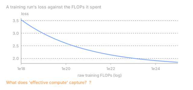
A scaling law is a fitted equation that predicts loss from parameters and training tokens. Kaplan (2020) said bigger model, lower loss. Hoffmann (2022) said those models were under-trained, and the split between parameters and tokens is the real decision.
Learning Objectives
- Split a fixed compute budget (C ≈ 6ND) between parameters and training tokens, and say what each knob buys.
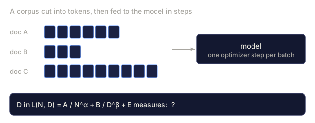
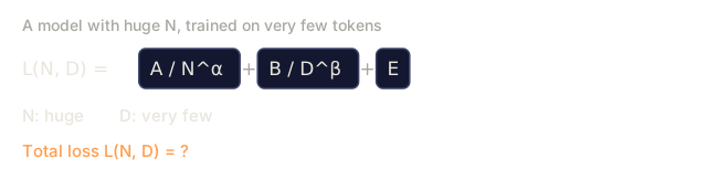
- Read the Hoffmann loss L(N, D) = A/N^α + B/D^β + E and explain what each term represents.
- Run a grid search for the compute-optimal (N, D) and explain why the fitted constants give a D/N that grows with C instead of a constant 20.
- Weigh the loss penalty of over-training against its inference savings for a heavily served model.
- Judge emergence claims and 2026 caveats (data quality, MoE, Muon) against smooth continuous loss.
The Problem
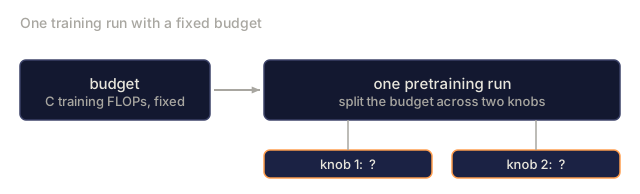
Compute-optimal scaling is the question of how to split a fixed training budget of C FLOPs between two knobs:
- Parameters (N). A bigger model has more capacity.
- Training tokens (D). More data makes better use of that capacity.
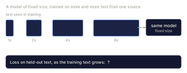
FLOPs scale approximately as 6 × N × D. You can push N up and D down, or D up and N down. Which gets you the lower loss?
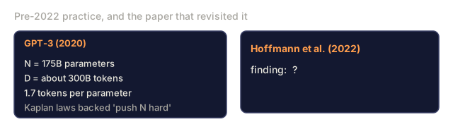
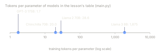
Before 2022 the answer was "push N hard." GPT-3 (2020) was 175B parameters trained on ~300B tokens, a ratio of about 1.7 tokens per parameter, and the Kaplan scaling laws backed that choice.
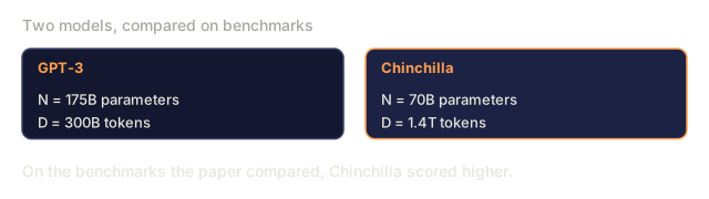
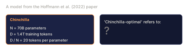
Hoffmann et al. (2022) trained a small family of models called Chinchilla and found a different optimum, closer to 20 tokens per parameter. By that measure GPT-3 was 10× undertrained. Chinchilla (70B params, 1.4T tokens) beat GPT-3 (175B, 300B tokens) on the benchmarks they compared, at 2.5× less inference cost.
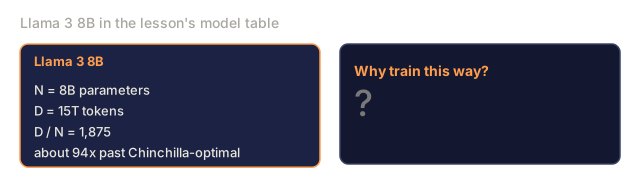
2026 is still Chinchilla's world, with one important twist. Llama 3 8B was trained on 15 trillion tokens, a ratio of 1,875 tokens per parameter, ninety-four times past Chinchilla-optimal. Inference cost matters more than training cost for a model that will be used at scale, so over-training past Chinchilla to get a smaller deployable footprint is the 2026 default.
The Concept

The Hoffmann law
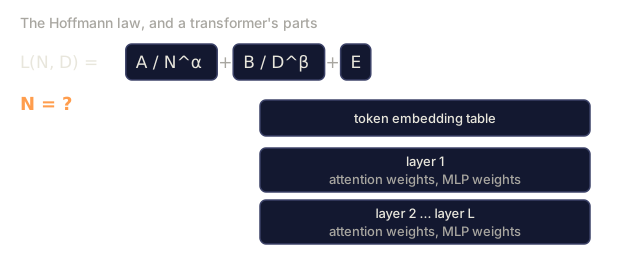
The Hoffmann law is a fitted formula for the loss of a model with N parameters trained on D tokens. From the Chinchilla paper:
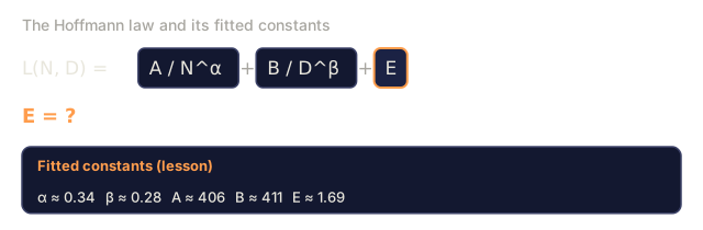
L(N, D) = A / N^α + B / D^β + E
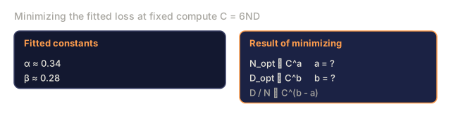
N= parameters (non-embedding).D= training tokens.α ≈ 0.34,β ≈ 0.28(roughly symmetric).E ≈ 1.69, the irreducible loss ceiling.A ≈ 406,B ≈ 411.
The two terms trade against each other as you scale. Substitute D = C / (6N) and minimize over N at fixed compute. Because α and β differ, the optimum is a power law in C with a different exponent for each knob:
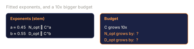
N_opt ∝ C^a,  a = β / (α + β) ≈ 0.45
D_opt ∝ C^b,  b = α / (α + β) ≈ 0.55
D_opt / N_opt ∝ C^(b - a) ≈ C^0.1
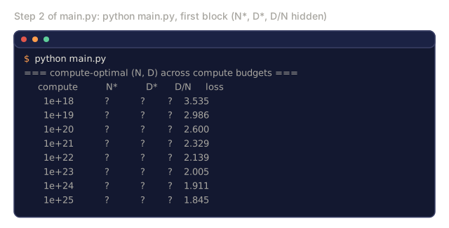
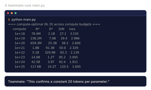
The prefactors depend on A and B. Since b > a, tokens per parameter creeps upward as compute grows instead of sitting at one constant. The grid search in main.py with the constants above prints about 27 tokens per parameter at 1e18 FLOPs, 65 at 1e22, 85 at 1e23, and 120 at 1e25. Published fits put the optimum near 20 tokens per parameter across the range Chinchilla studied (roughly 1e22 to 1e23 FLOPs), and that is the headline number to remember. The fitted constants here don't reproduce it exactly.
Why over-training anyway
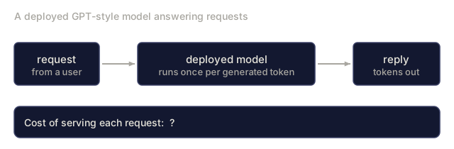
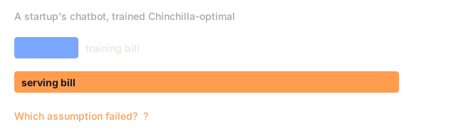
Chinchilla-optimal minimizes training loss per training FLOP. But you pay training cost once, and you pay inference cost for as long as the model is served.
For a chatbot that serves a trillion tokens per month, inference dominates total cost. Llama's approach is to train smaller and longer. 8B at 15T tokens is deeply inference-optimized:
- It fits on consumer GPUs.
- Latency is a fraction of a 70B Chinchilla-optimal model.
- Quality is close enough for most tasks.
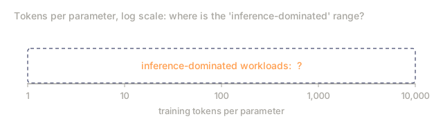
DeepMind's 2024 paper ("Over-training is the new optimal") formalized this. For inference-dominated workloads, the right ratio is closer to 100–500 tokens per parameter depending on serving volume.
Emergence vs smoothness
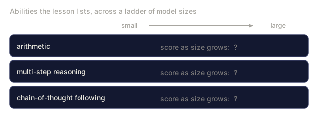
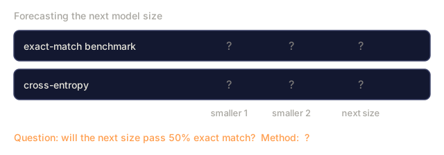
Emergence is the claim that certain abilities (arithmetic, multi-step reasoning, chain-of-thought following) appear suddenly at some scale.
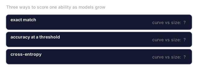
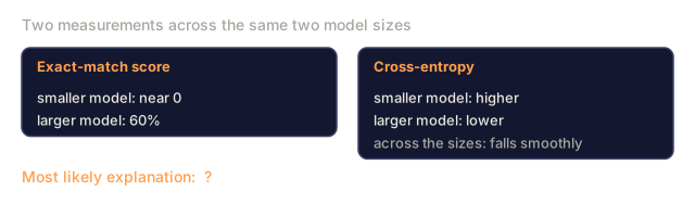
Schaeffer et al. (2023) argued this is a measurement artifact. Emergent metrics use discontinuous scoring (exact match, accuracy at threshold), which hides smooth improvement in the underlying logits. Continuous metrics such as cross-entropy show smooth curves.
In 2026 the consensus is that predictions via continuous loss are reliable, and benchmark jumps are often scorer artifacts. Plan budgets against continuous metrics.
The 2026 picture
Scaling laws still work, with some caveats:
| Factor | Changed how |
|---|---|
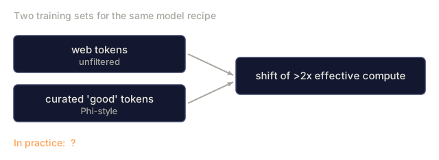
| Data quality | Curating "good" tokens (Phi-style) shifts curves by >2× effective compute |
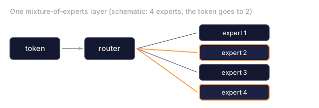
| MoE | Total params decouple from active FLOPs; scaling laws per-active-FLOP |
| Post-training | Some capabilities (instruction following, code) shift with SFT+RLHF more than pretraining |
| Multimodality | Image + text tokens scale together; separate curves per modality |
| Synthetic data | Models generate training data; effective compute can compound |
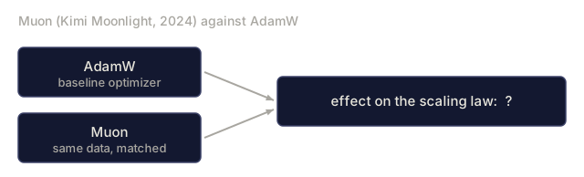
The Muon optimizer (Kimi Moonlight, 2024) showed a ~2× effective-compute gain over AdamW at matched data. Some 2026 training runs use Muon by default. It changes the absolute constant in the scaling law, not its shape.

Build It
The code is in code/main.py. It implements the Chinchilla loss equation and solves for compute-optimal (N, D) at each of several compute budgets.
Step 1: Chinchilla loss
def chinchilla_loss(N, D, A=406.4, B=410.7, alpha=0.34, beta=0.28, E=1.69):
    return A / N ** alpha + B / D ** beta + E
main.py has no plotting. To see the valley yourself, evaluate L on an (N, D) grid and draw a contour (matplotlib's contourf works). The minimum along any fixed C = 6ND line is what Step 2 searches for.
Step 2: compute-optimal frontier
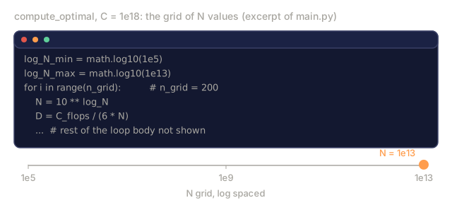
For eight compute budgets, one per decade from 1e18 to 1e25 FLOPs, compute_optimal finds the (N, D) that minimizes loss subject to 6ND = C. It grid-searches 200 log-spaced values of N from 1e5 to 1e13, sets D = C / (6N), skips any point with D < 1e6, and keeps the lowest loss. Then check the ratio D/N. With these fitted constants it is not constant: the printed optimum is 27.1 at 1e18, 29.4, 38.3, 50.0, 65.3 at 1e22, 85.2 at 1e23, 92.4, and 120.5 at 1e25. The printout notes that published fits put it near 20 for the Chinchilla range, so treat 20 as a published headline, not something this code reproduces.
Step 3: over-training cost
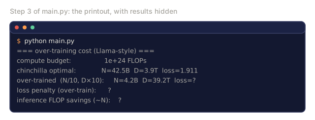
Fix C = 1e24, take the compute-optimal (N_opt, D_opt), then compute the extra loss you pay to train a 10× smaller model (N_opt / 10, 10 × D_opt, which spends the same compute). Report the inference FLOP savings (proportional to N) you get in exchange. main.py prints a loss penalty of +0.059 for a 10× inference saving.
Step 4: compare to real models
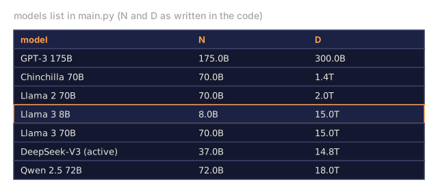
main.py drops in known (N, D) pairs for seven models: GPT-3 175B, Chinchilla 70B, Llama 2 70B, Llama 3 8B, Llama 3 70B, DeepSeek-V3 (active params), and Qwen 2.5 72B. It prints each model's D/N and the loss the fitted equation predicts, nothing else. If you want a predicted-vs-reported comparison, add the reported losses yourself.
Use It
You're unlikely to train a frontier model yourself. Scaling laws still tell you three things:
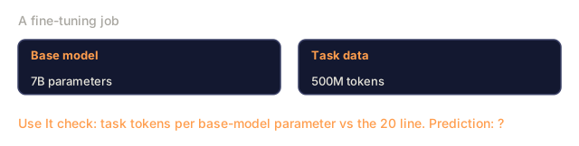
- Whether your fine-tune has enough data. If your task-specific data is below 20 tokens per param of the base model, expect saturation at some loss floor.
- Whether to pick a bigger base model. If you're spending your whole budget on inference, prefer a smaller, longer-trained model.
- Where the returns diminish. Beyond 1000× Chinchilla-optimal, log-loss changes become noise.
The research trajectory in 2026:
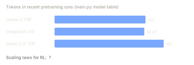
- Data-constrained regime. The web has a finite number of high-quality tokens (~5–10 trillion English after filtering), and frontier pretraining is approaching that ceiling. Synthetic data, multilingual, multimodal, and RLHF-scaled fine-tuning are the next levers.
- Compute-multiplier tricks. Muon optimizer, MoE, and better data curation each shift the absolute constants, not the asymptote.
- Scaling laws for RL. Still an open question. Early evidence suggests a power law in RL samples, but with very different exponents than pretraining.
Ship It
The skill in outputs/skill-training-budget-estimator.md picks (N, D, hours, GPU) for a new training run given a compute budget, deployment constraints, and a target loss.
I'd treat the 20 tokens per parameter figure as a number to check, not a constant to memorize. The formulas in The Concept give N_opt and D_opt the same expression, which can't produce a ratio of 20 on its own. main.py grid-searches the fitted constants instead, and the optimum D/N it finds grows with C: about 27 at 1e18, 65 at 1e22, and 85 at 1e23. Its printout notes that published fits put the optimum near 20 for the range Chinchilla studied, so the fitted constants here and the headline ratio don't agree.
My bet is that the over-training step is the most useful one to run for your own numbers. It takes the 1e24 budget, shrinks N by 10×, grows D by 10×, and prints the loss penalty next to the inference savings (about N_opt / N_under, so 10x). Set that trade against how much serving you expect, since the case for Llama-style training rests on inference volume.
I'd also read the real-model table as predicted loss from the fitted equation, not as a comparison against published numbers. main.py prints chinchilla_loss for each model and has no reported-loss column, so Step 4's "predicted vs reported" is a comparison you'd add yourself.
Exercises
- Easy. Run
code/main.py. Print Chinchilla-optimal(N, D)for compute budgets1e20,1e22,1e24. Compare to the real model table. - Medium. Implement the Hoffmann loss-as-function-of-compute curve. Plot loss vs
log10(C)for the compute-optimal frontier. Identify when the law predicts we'd need>10^28FLOPs for the next 0.1 reduction in cross-entropy. - Hard. Fit your own scaling law on 5 tiny models (100K to 10M params) trained on the same dataset. Estimate
αandE. How well do your exponents match published ones?
Key Terms
| Term | What people say | What it actually means |
|---|---|---|
| Parameters (N) | "Model size" | Non-embedding weight count; determines capacity. |
| Tokens (D) | "Training data" | Number of training tokens seen; determines how well the parameters get used. |
| Compute (C) | "FLOPs spent" | Approximately 6 × N × D for a standard transformer. |
| Chinchilla-optimal | "D/N ≈ 20" | Ratio that minimizes loss per FLOP of pretraining. Published fits put it near 20; the fitted constants in this lesson give a ratio that grows with C. |
| Over-training | "Past Chinchilla" | Spend extra training FLOPs to save inference FLOPs; D/N >> 20. |
| Irreducible loss | "The floor" | The E term in the scaling law; the entropy of the data itself. |
| Emergent capability | "Sudden jumps at scale" | Often a scorer artifact; continuous loss is smooth. |
| Effective compute | "Training-efficiency multiplier" | Better data / optimizer / architecture multiplies how far a FLOP goes. |
Further Reading
- Kaplan et al. (2020). Scaling Laws for Neural Language Models: the first scaling law paper, and under-trained by Hoffmann's measure.
- Hoffmann et al. (2022). Training Compute-Optimal Large Language Models: Chinchilla.
- Schaeffer et al. (2023). Are Emergent Abilities of Large Language Models a Mirage?: emergence as measurement artifact.
- Sardana, Frankle (2024). Beyond Chinchilla-Optimal: Accounting for Inference in Language Model Scaling Laws: why Llama's over-training suits its workload.
- Jordan et al. (2024). Muon: An optimizer for hidden layers in neural networks: 2× compute multiplier.
Code
- main.py (python, 95 lines)