TAI BUI
Back to curriculum
LearnPython

Why Transformers — The Problems with RNNs

RNNs read tokens one at a time. Transformers read all of them at once. That one architectural bet reshaped the scaling curves of deep learning after 2017.

TIME: ~45 minutesPREREQUISITES: Phase 3 (Deep Learning Core), Phase 5 · 09 (Sequence-to-Sequence), Phase 5 · 10 (Attention Mechanism)

Learning Objectives

  • Name the three weaknesses of RNNs (serial computation, vanishing gradients, a fixed-width hidden state) that motivated the transformer.
  • Compare the serial dependency depth of a recurrence with a parallel reduction and a prefix scan, using the depth table that `main.py` prints.
  • Explain the O(N²) memory cost of self-attention and why parallelism still wins back wall-clock time.
  • Decide when an RNN, a state-space model, a hybrid, or a transformer is the right choice for a sequence problem.

The Problem

A recurrent neural network (RNN) reads a sequence one token at a time, folding each token into a hidden state that it carries forward to the next step. Before 2017, that was the architecture behind the leading models for language, translation, and speech. LSTMs and GRUs led translation benchmarks for roughly half a decade, and nothing else seriously competed.

They had three weaknesses, and each one hurt.

Sequential computation meant you could not parallelize along the time axis: token t+1 needs the hidden state from token t. A 1,024-token sequence meant 1,024 serial steps on a GPU that can do 1,000,000 floating-point ops per cycle. Training wall-clock time grew linearly with sequence length, on hardware built for parallelism.

Vanishing gradients meant information 50 tokens back had already passed through 50 non-linearities. Gated recurrent units (LSTM, GRU) softened the crush but did not remove it. Long-range dependencies, like "the book I read last summer on a plane to Kyoto was…", routinely failed.

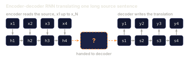
Fixed-width hidden states meant the encoder squeezed the whole source sequence into a single vector before the decoder saw anything. Whether the source is 5 tokens or 500, the bottleneck has the same shape.

The 2017 paper "Attention Is All You Need" dropped recurrence entirely. All positions attend to all other positions in parallel, and training becomes one big matrix multiplication instead of 1,024 sequential ones.

By 2026 the same block runs across modalities: language (GPT-5, Claude 4, Llama 4), vision (ViT, DINOv2, SAM 3), audio (Whisper), biology (AlphaFold 3), robotics (RT-2). Same block, different inputs.
Warm-up0/3
1. In a basic encoder-decoder RNN for translation (Phase 5 · 09), what limits how much of a long source sentence the decoder can use?Warm-up
An encoder RNN on the left with inputs x1 to x4 (and on to x_N) and hidden states h1 to h4, a dashed box with a question mark labelled handed to decoder in the middle, and a decoder RNN on the right with states s1 to s4 and outputs y1 to y4.
Schematic of the setup in the stem. The dashed box is what the question asks about.
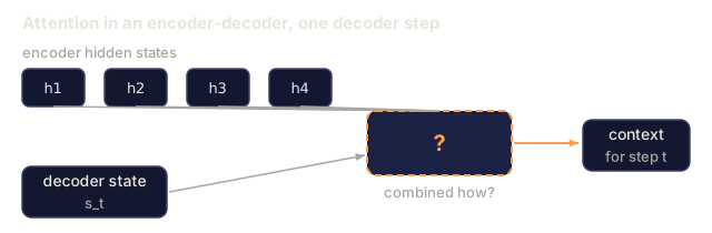
2. In the attention mechanism from Phase 5 · 10, how does the decoder combine the encoder's hidden states at each step?Warm-up
Four encoder hidden states h1 to h4 and a decoder state s_t both feed a dashed box with a question mark labelled combined how, which produces the context for step t.
Schematic. The dashed box is what the stem asks about.
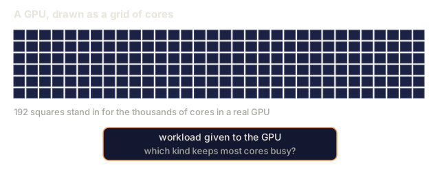
3. A GPU has thousands of cores. Which kind of workload keeps most of them busy?Warm-up
A grid of 192 small squares representing GPU cores, with a box below reading workload given to the GPU, which kind keeps most cores busy.
Schematic, not to scale.
Check: The Problem0/3
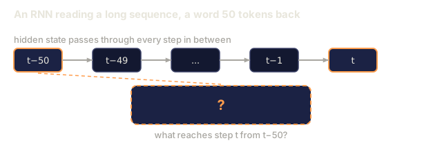
1. Why does a long-range dependency, like a word 50 tokens back, often fail in an RNN?Explain
A chain of boxes t−50, t−49, dots, t−1 and t joined by arrows, with t−50 and t highlighted, and a dashed box with a question mark labelled what reaches step t from t−50.
Schematic of the stem's setup. The dashed box is what the question asks about.
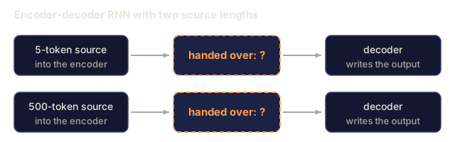
2. Why does a fixed-width hidden state hurt an encoder-decoder RNN on a 500-token source?Explain
Two rows, a 5-token source and a 500-token source, each going into the encoder, then a dashed box with a question mark labelled handed over, then the decoder.
Schematic. The dashed boxes are what the question asks about.
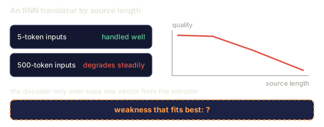
3. An RNN translator handles 5-token inputs well but degrades steadily at 500 tokens, and its decoder only ever sees one vector from the encoder. Which weakness fits best?Analyze
Two rows, 5-token inputs handled well and 500-token inputs degrading steadily, a sketched falling quality curve against source length, a note that the decoder only sees one vector from the encoder, and a dashed box reading weakness that fits best: question mark.
Qualitative sketch of the symptom in the stem; no measured data.

The Concept

RNN sequential compute vs Transformer parallel attention

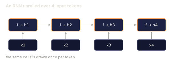
Recurrence is computation where step t depends on step t-1. An RNN computes h_t = f(h_{t-1}, x_t), so you cannot compute h_5 before h_4. On a modern GPU with 10,000+ parallel cores, that wastes 99% of the silicon on a long sequence.

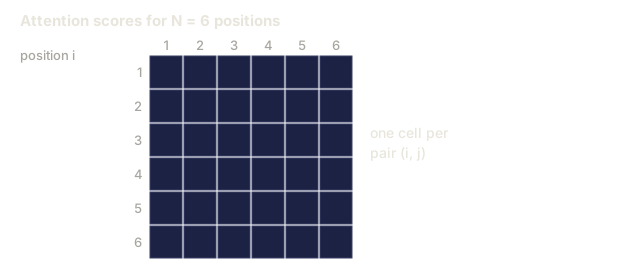
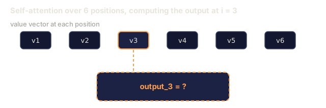
Self-attention is a weighted sum over the whole sequence: output_i = sum_j(a_ij * v_j), computed for all pairs (i, j) at once. The full N×N attention matrix fills in one batched matmul, and no step waits on another. That is the shape GPUs are built for.

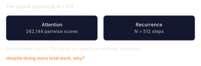
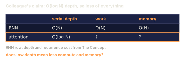
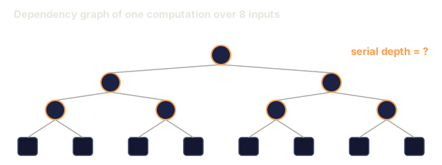
The speedup is not a constant. It is the difference between O(N) serial depth and O(log N) serial depth, since a tree reduction combines N values in log N rounds. In practice, transformers train 5–10× faster per epoch on matched hardware at N=512, and the gap widens with sequence length until you hit the O(N²) memory wall of attention (Flash Attention later attacked that wall, see Lesson 12).

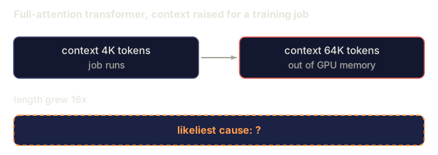
What transformers cost. Attention memory scales as O(N²). At 2K context that is fine. At 128K you need sliding windows, RoPE extrapolation, Flash Attention tiling, or linear attention variants. Recurrence was O(N) in both time and memory. Attention does O(N²) work and holds O(N²) memory, and parallelism wins the wall-clock time back.

The inductive bias shift. RNNs assume locality and recency. Transformers build in no such assumption: all pairs are candidates for attention. That is why transformers need more data to train well but scale further once they have it. Chinchilla (2022) formalized this: given enough tokens, a transformer beats an RNN of equal parameter count.
Check: The Concept0/13
1. What is recurrence in a sequence model?Define
An RNN unrolled over four tokens: inputs x1 to x4 along the bottom, a box f producing hidden state h1 to h4 above each input, and an arrow from each box into the next.
A concrete instance of a recurrent model.
2. What is attention, as the lesson defines it?Define
Six position boxes v1 to v6 with position 3 highlighted, and a dashed line down to a box reading output_3 equals question mark.
Schematic for position i = 3 of 6. The dashed box is what the question asks about.
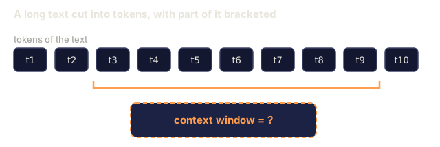
3. What is a context window?Define
A row of ten token boxes t1 to t10 with a bracket under t3 to t9 and a dashed box below reading context window equals question mark.
Schematic with 10 tokens. The dashed box is what the question asks about.
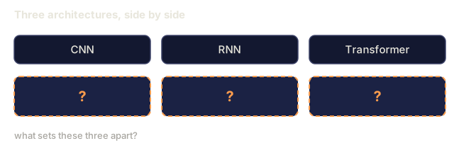
4. What is an inductive bias?Define
Three cards named CNN, RNN and Transformer, each with a dashed box holding a question mark, under the line what sets these three apart.
Each dashed box is what the question asks about.
5. What is the quadratic bottleneck of attention?Define
A six by six grid of cells with positions 1 to 6 on both axes, labelled one cell per pair (i, j).
Concrete instance for N = 6: the N x N attention matrix.
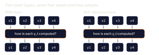
6. What is the key mathematical difference between how an RNN and self-attention compute outputs?Explain
Two panels, RNN layer and Self-attention layer, each taking inputs x1 to x4 into a box asking how each y_t is computed and producing outputs y1 to y4.
Schematic. The boxes are what the question asks about.
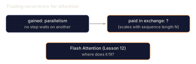
7. What cost does the lesson say attention pays in exchange for parallelism, and where does Flash Attention fit?Explain
A box reading gained: parallelism, an arrow to a dashed box reading paid in exchange: question mark scales with sequence length N, and below it a box asking where Flash Attention from Lesson 12 fits.
Schematic. The accented boxes are what the question asks about.
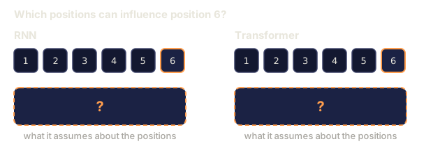
8. How does the lesson describe the inductive-bias difference between RNNs and transformers?Explain
Two panels, RNN and Transformer, each showing six positions 1 to 6 with position 6 highlighted and a dashed box with a question mark labelled what it assumes about the positions.
Schematic. The dashed boxes are what the question asks about.
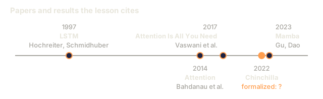
9. What does the lesson say Chinchilla (2022) formalized about the transformer and RNN comparison?Explain
A timeline with 1997 LSTM, 2014 Attention, 2017 Attention Is All You Need, 2022 Chinchilla marked with formalized: question mark, and 2023 Mamba.
Years and names from the lesson's Further Reading and The Concept.
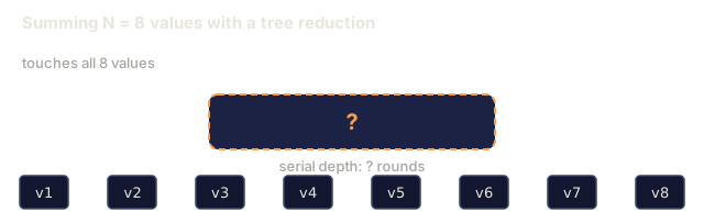
10. Why is a tree reduction O(log N) in serial depth even though it touches all N values?Explain
Eight value boxes v1 to v8 with a dashed box with a question mark above them labelled serial depth: question mark rounds.
Schematic. The dashed box is what the question asks about.
11. Attention does O(N²) work, yet transformers train faster than RNNs at N=512. Why?Explain
Two boxes: attention with 262,144 pairwise scores at N = 512, and recurrence with 512 steps, followed by a line noting transformers train 5 to 10 times faster per epoch despite more total work.
Entry count is 512 x 512. The 5-10x figure is the lesson's.
12. Your team raises a full-attention transformer's context from 4K to 64K tokens and the job runs out of GPU memory. What is the likeliest cause?Analyze
A box for context 4K tokens where the job runs, an arrow to a box for context 64K tokens that runs out of GPU memory, the note length grew 16x, and a dashed box reading likeliest cause: question mark.
Setup from the stem. The dashed box is what the question asks about.
13. A colleague says transformers need only O(log N) serial depth, so they must also use less compute and memory than RNNs. What is wrong with that?Analyze
A table for RNN and attention with columns serial depth, work and memory. RNN is O(N) in all three; attention has O(log N) depth and question marks for work and memory.
Entries from The Concept. The question marks are what the question asks about.

Build It

This build has no neural network. We simulate the core bottleneck numerically so you can feel the gap on your laptop.

Step 1: measure serial depth

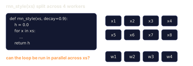
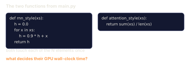
See code/main.py. It defines two functions. One is a decayed recurrence (serial, like an RNN): each step multiplies the previous state by 0.9 and adds the new element. The other is a plain mean over the sequence (order-independent, like the reduction inside attention). Same input, different dependency graph.

python
def rnn_style(xs):
    h = 0.0
    for x in xs:
        h = 0.9 * h + x   # can't parallelize: h depends on previous h
    return h
 
def attention_style(xs):
    return sum(xs) / len(xs)  # every x is independent

We time both at N = 1,000, 10,000, 100,000, and 1,000,000. The RNN version is O(N) and runs down a single CPU pipeline. Even in pure Python, the attention-style reduction beats it at every one of those lengths, because Python's sum() is implemented in C and iterates without interpreter overhead per step.

Step 2: count theoretical operations

Both functions touch each of the N elements once. What differs is dependency depth: how many operations must happen sequentially before the next can start. RNN depth = N. Attention-style depth = ceil(log2 N) with a tree reduction, which is what depth() in main.py computes. The script's parallel_scan (a Hillis-Steele prefix sum) has the same O(log N) depth, and the script checks it against serial_scan on a length-16 sequence (zero mismatches, last value 120.0). Depth, not op count, decides GPU time.

Step 3: empirical scaling on long sequences

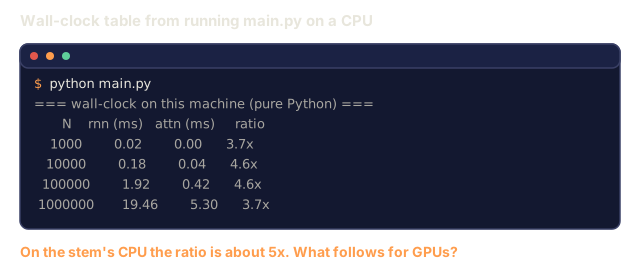
The script prints two tables. The depth table runs N from 64 to 262,144: RNN depth grows from 64 to 262,144 while attention-style depth grows from 6 to 18. The wall-clock table is the noisier one. On one run, the RNN loop took about 0.03 ms at N = 1,000 and about 31 ms at N = 1,000,000, with the attention-style reduction 4 to 7 times faster at each length. Your numbers will differ. That gap is mostly interpreter overhead, so read the depth table for the architectural claim.
Check: Build It0/8
1. What does serial depth measure?Define
A dependency graph: eight input boxes at the bottom, four circles above them, then two, then one, with lines showing which results feed which operation, and the label serial depth equals question mark.
A concrete computation (a sum of 8 values) drawn as a dependency graph.
2. `rnn_style` and `attention_style` both touch each of the N elements once. What decides GPU wall-clock time between them?Explain
The source of rnn_style, a loop that updates h from 0.9 times h plus x, next to attention_style, which returns sum(xs) divided by len(xs).
Code copied from the lesson's main.py.
3. In the lesson's code, why can't `rnn_style(xs)` be parallelized across the sequence?Apply
The signature of rnn_style with its loop body hidden as dots, eight elements x1 to x8 in two rows, and four worker boxes w1 to w4, with the question of whether the loop can run in parallel across xs.
The loop body is hidden on purpose. Signature from main.py.
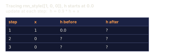
4. What does `rnn_style([1, 0, 0])` return, given `h = 0.9 * h + x` starting from h = 0.0?Apply
A trace table for rnn_style on the list 1, 0, 0 with columns step, x, h before and h after. The first row has x = 1 and h before 0.0; the remaining h cells are question marks.
Setup from the stem. Question marks are the values to work out.
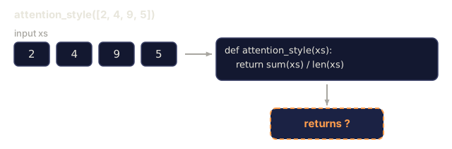
5. What does `attention_style([2, 4, 9, 5])` return?Apply
The list 2, 4, 9, 5 going into attention_style, whose source is return sum(xs) / len(xs), with a dashed box reading returns question mark.
Source copied from main.py. The dashed box is what the question asks about.
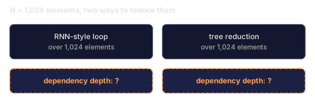
6. For N = 1,024, what dependency depths do the RNN-style loop and a tree reduction have?Apply
Two boxes, an RNN-style loop and a tree reduction, both over 1,024 elements, each with a dashed box below reading dependency depth: question mark.
The dashed boxes are what the question asks about.
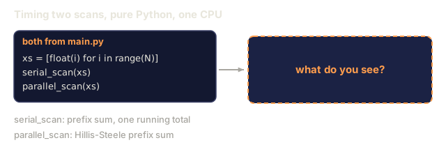
7. You time `parallel_scan` against `serial_scan` in pure Python on a CPU. What should you expect?Apply
A code box listing a list xs, serial_scan(xs) and parallel_scan(xs), an arrow to a dashed box reading what do you see, and two lines naming serial_scan as a prefix sum with one running total and parallel_scan as a Hillis-Steele prefix sum.
Function names from main.py. The dashed box is what the question asks about.
8. You run `main.py` and the attention-style reduction is about 5x faster than `rnn_style` on your CPU. What should you conclude about GPUs?Analyze
A terminal showing the wall-clock table of main.py with N from 1000 to 1000000, rnn and attn times in milliseconds and the ratio, followed by the question of what follows for GPUs.
Cached capture of main.py on the sandbox CPU; ratios are about 4x, a bit under the stem's 5x, and vary by run.

Use It

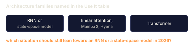
When to still pick an RNN in 2026:

SituationPick
Streaming inference, one token at a time, constant memoryRNN or state-space model (Mamba, RWKV)
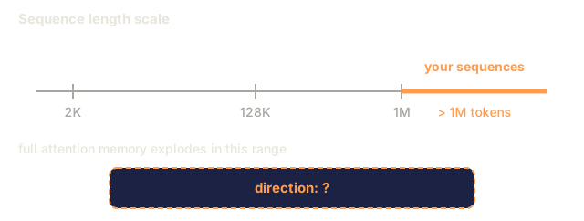
Very long sequences (>1M tokens) where attention memory explodesLinear attention, Mamba 2, Hyena
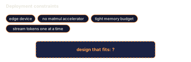
Edge device with no matmul acceleratorDepthwise-separable RNN still wins on FLOPs/watt
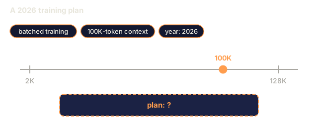
Anything else (training, batched inference, context up to 128K)Transformer

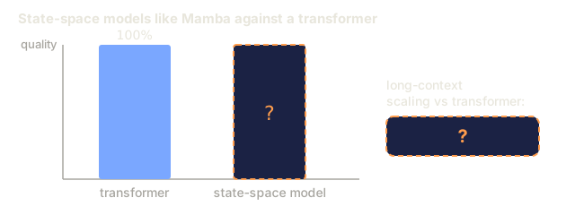
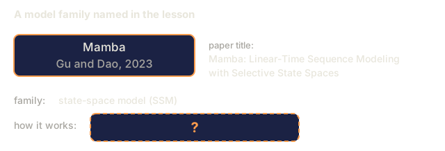
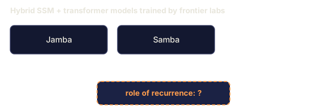
State-space models (SSMs) like Mamba are essentially RNNs with a structured parameterization that gives them the best of both: O(N) scan memory and parallel training via selective scan. They recover 90% of transformer quality with better long-context scaling. In 2026 most frontier labs train hybrid SSM+transformer models (Jamba, Samba), so recurrence has become a component rather than a rival.
Check: Use It0/6
1. What is a state-space model such as Mamba?Define
A card for Mamba (Gu and Dao, 2023) with the paper title Mamba: Linear-Time Sequence Modeling with Selective State Spaces, the family state-space model, and a dashed box with a question mark for how it works.
Names and paper title from the lesson's Further Reading. The dashed box is what the question asks about.
2. Hybrid SSM+transformer models like Jamba and Samba are now trained by frontier labs. What does that imply about recurrence?Explain
Two boxes named Jamba and Samba, and a dashed box reading role of recurrence: question mark.
Names from the Use It section. The dashed box is what the question asks about.
3. How do state-space models like Mamba compare to transformers in quality, per Use It?Explain
A bar chart with a transformer bar at 100 percent and a dashed state-space bar with a question mark for quality, plus a dashed box with a question mark for long-context scaling versus the transformer.
The transformer is the reference at 100%. The dashed shapes are what the question asks about.
4. Per the Use It table, which situation should still lean toward an RNN or state-space model in 2026?Apply
Three boxes: RNN or state-space model, linear attention with Mamba 2 and Hyena, and Transformer, with the question of which situation should still lean toward an RNN or state-space model in 2026.
Family names from the lesson's Use It table.
5. You must stream tokens one at a time on an edge device with no matmul accelerator and a tight memory budget. Which design fits?Design
Four constraint chips, edge device, no matmul accelerator, tight memory budget and stream tokens one at a time, above a dashed box reading design that fits: question mark.
Constraints copied from the stem.
6. Your sequences run past 1M tokens, where full attention memory explodes. Which direction does the lesson point to?Design
A number line of sequence length with ticks at 2K, 128K and 1M, the range beyond 1M tokens highlighted and labelled your sequences, the note that full attention memory explodes there, and a dashed box reading direction: question mark.
Scale marks from the lesson; positions are not to scale.

Ship It

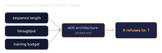
See outputs/skill-architecture-picker.md. The skill picks an architecture for a new sequence problem given length, throughput, and training-budget constraints. It refuses to recommend a pure RNN for a training run above 1B tokens until it has stated the trade-off. It also refuses to recommend full attention above 64K context without stating the O(N²) memory cost, and refuses to recommend an architecture published less than 12 months ago for production without a named fallback.
Check: Ship It0/2
1. Per Ship It, what must the architecture-picker skill refuse to do?Explain
Three input boxes, sequence length, throughput and training budget, feeding a box named skill-architecture-picker.md, which points to a dashed box reading it refuses to: question mark.
Inputs and file name from Ship It. The dashed box is what the question asks about.
2. You plan batched training on a 100K-token context in 2026. Which plan matches the lesson's guidance?Design
Three chips, batched training, 100K-token context and year 2026, a scale from 2K to 128K with a marker at 100K, and a dashed box reading plan: question mark.
Setup from the stem. Marker position is to scale between 2K and 128K.
Author's Note

I'd read the depth table before the wall-clock table. The wall-clock numbers mostly measure Python's per-step loop overhead against a sum() that runs in C, which says little about GPUs. The depth table is the actual claim about architecture. The script's own parallel_scan docstring is blunt about this: in pure Python each step is still serial, so the time on a CPU does not improve, and what changes is the shape of the dependency graph.

I'd also treat attention_style as a stand-in for dependency structure and nothing more. It is a mean over the input and has no a_ij weights, so it shows you what independence looks like without showing you attention. The real mechanism arrives in the next lessons.

My bet is that the hybrid line in Use It is the part that ages best. Pure RNN versus pure transformer is a framing from 2017, and the table of situations where recurrence still wins is a reason to keep both in your toolbox.

Exercises

  1. Easy. Take rnn_style from code/main.py and replace the scalar hidden state with a length-64 vector of hidden states. Re-measure. How much does the serial overhead grow with hidden-state dimension?
  2. Medium. Extend the parallel_scan and serial_scan equivalence check in code/main.py, which only runs at length 16. Verify the two produce the same output on length 1024, then instrument parallel_scan to count its rounds and confirm the depth is log2(N).
  3. Hard. Port the attention-style reduction to PyTorch on GPU. Time both as you sweep sequence length from 64 to 65,536. Plot the result and explain the curve shape.

Key Terms

TermWhat people sayWhat it actually means
Recurrence"RNNs are sequential"Computation where step t depends on step t-1, forcing serial execution along the time axis.
Serial depth"How deep the graph is"Longest chain of dependent ops; bounds wall-clock even on infinite hardware.
Attention"Let tokens look at each other"Weighted sum sum_j a_ij v_j where a_ij comes from a similarity score between positions i and j.
Context window"How much the model sees"Number of positions an attention layer can take as input; quadratic memory cost scales here.
Inductive bias"Assumptions baked into the architecture"Prior about what the data looks like; CNNs assume translation invariance, RNNs assume recency.
State-space model"RNN with algebra behind it"Recurrence parameterized for parallel training via structured state-space matrices.
Quadratic bottleneck"Why context costs so much"Attention memory = O(N²) in sequence length; Flash Attention hides the constants, not the scaling.

Further Reading

Code

Ships With