Attention Variants — Sliding Window, Sparse, Differential
Full attention scores each token against the whole prefix, and memory pays the price. Four variants change which pairs get scored, or how the scores combine, and recover half the cost.
Learning Objectives
- Describe how sliding window, sparse, and differential attention each change which query-key pairs get scored or how the weights combine.
- Build causal, sliding-window, and local+strided masks in plain Python and read them as 8-token grids.
- Explain the attention sink and how subtracting a second attention map targets it.
- Estimate KV cache size at 128K context for full, SWA, 5:1 mixed, and differential attention.
- Choose between full, SWA plus global, sparse, and differential attention for a given context length and retrieval need.
The Problem
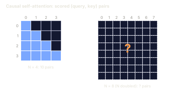
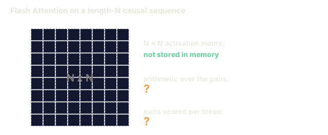
Full attention costs O(N²) memory and O(N²) compute in sequence length. For a 128K-context Llama 3 70B that is 16 billion attention entries per layer, times 80 layers. Flash Attention (Lesson 12) hides the O(N²) activation memory but does not change the arithmetic cost: each token still attends to the full prefix.
An attention variant is a change to the structure of the attention matrix: which (query, key) pairs get scored, or how the resulting weights are combined. Three classes of variants do this:
- Sliding window attention (SWA). Each token attends to a fixed window of neighbors instead of the full prefix. Memory and compute drop to
O(N · W)whereWis the window. Used in Gemma 2/3, Mistral 7B's first layers, and Phi-3-Long. - Sparse / block attention. Only selected pairs
(i, j)get scored, and the rest are forced to zero weight. Longformer, BigBird, and the OpenAI sparse transformer work this way. - Differential attention. Compute two attention maps with separate Q/K projections and subtract one from the other. The subtraction targets the "attention sink" that bleeds weight into the first few tokens. This is Microsoft's DIFF Transformer (2024).
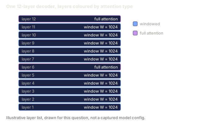
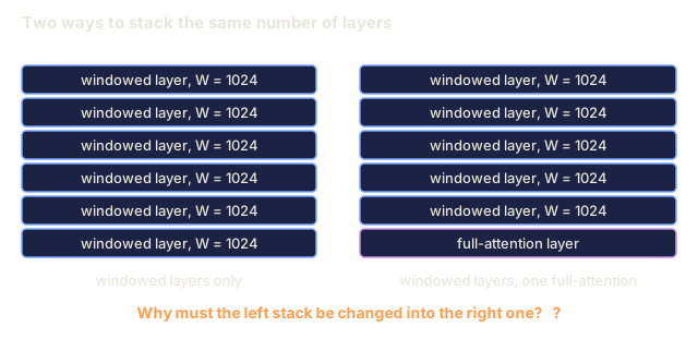
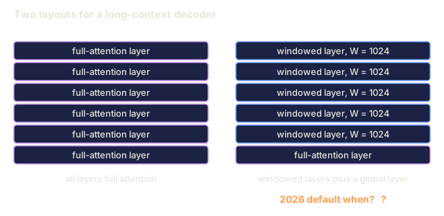
These can be combined. A 2026 frontier model often mixes them: most layers are SWA-1024, a periodic layer is global full attention, and a handful are differential heads that clean up retrieval. Gemma 3's 5:1 SWA-to-global ratio is the current textbook default.
The Concept
Sliding Window Attention (SWA)
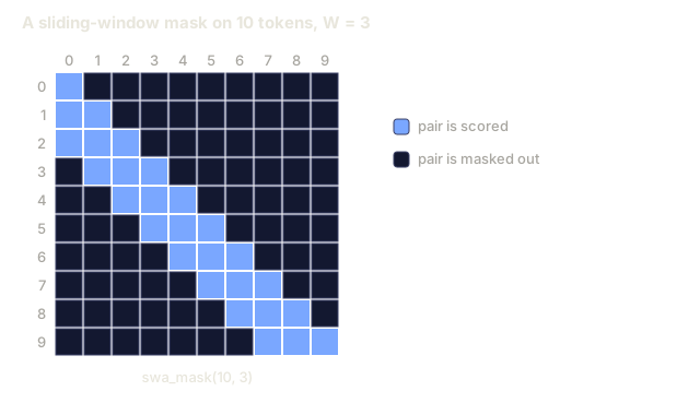
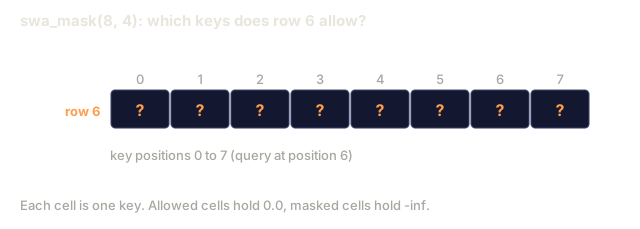
Sliding window attention limits each query at position i to the positions in [i - W, i] (causal SWA) or [i - W/2, i + W/2] (bidirectional). Tokens outside the window get -inf in the score matrix.
full causal:           sliding window (W=4):
positions 0-7          positions 0-7, W=4
    0 1 2 3 4 5 6 7        0 1 2 3 4 5 6 7
0 | x                0 |  x
1 | x x              1 |  x x
2 | x x x            2 |  x x x
3 | x x x x          3 |  x x x x
4 | x x x x x        4 |    x x x x
5 | x x x x x x      5 |      x x x x
6 | x x x x x x x    6 |        x x x x
7 | x x x x x x x x  7 |          x x x x
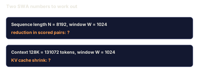
For N = 8192 and W = 1024, each of the 8192 queries scores at most 1024 keys instead of up to 8192, an 8× reduction in scored pairs.
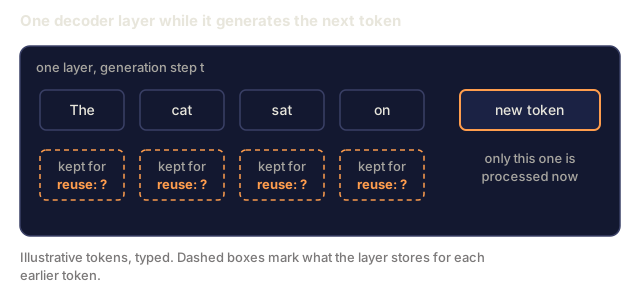
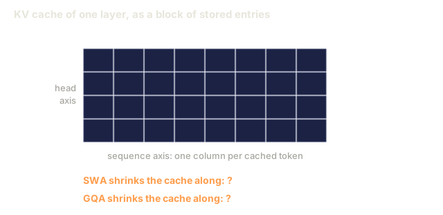
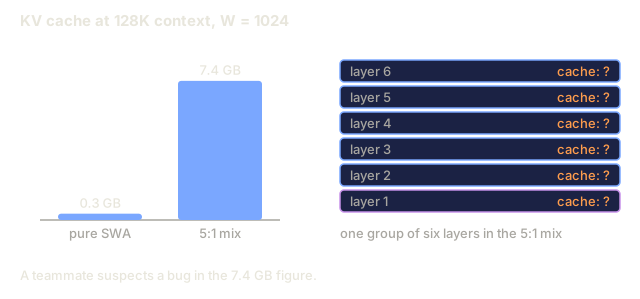
KV cache shrinks with SWA. Only the last W tokens of K and V need to be kept per layer. For a Gemma-3-ish config (1024 window, 128K context), KV cache drops 128×.
SWA shrinks the cache along the sequence axis. Grouped-query attention (GQA, Lesson 03) shrinks it along the head axis by letting several query heads share one K/V head, and the two savings can be combined. The figure below shows the head-axis side.
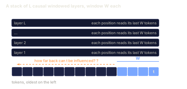
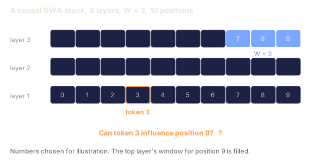
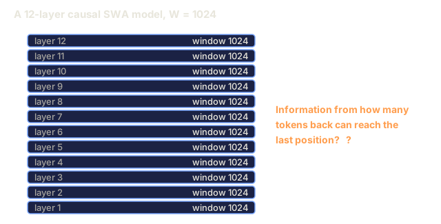
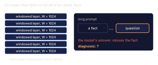
Quality cost. SWA-only transformers struggle with long-range retrieval. The fix is to interleave SWA layers with full-attention layers, and Gemma 3 uses 5:1 SWA:global. Mistral 7B used a causal-SWA stack where information "flows forward" through overlapping windows. Each layer extends the effective receptive field by W, so after L layers the model can attend L × W tokens back.
Sparse / Block Attention
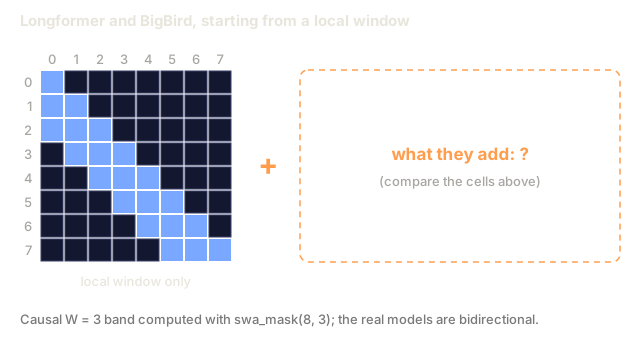
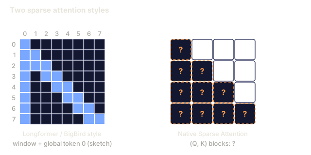
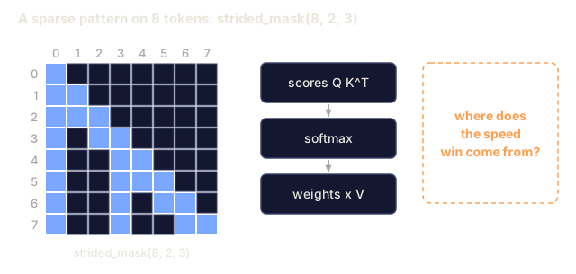
Sparse attention scores a pre-chosen subset of (i, j) pairs and gives the rest zero weight. You pick an N × N sparsity pattern ahead of time. Three canonical shapes:
- Local + strided (OpenAI sparse transformer). Attend to the last
Wtokens plus everystride-th token before that. This captures both local and long-range structure atO(N · sqrt(N))compute. - Longformer / BigBird. A local window, plus a small set of global tokens (e.g.
[CLS]) that attend to everyone and are attended by everyone, plus random-sparse links. Empirically this gives 2× context at matched quality. - Native Sparse Attention (DeepSeek, 2025). Learn which blocks of
(Q, K)matter, and skip the zero blocks at kernel level. It stays FlashAttention-compatible.
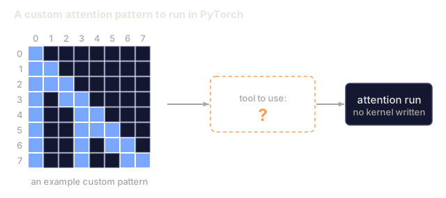
Sparse attention is a kernel-engineering story. The math is simple (mask the score matrix), and the win comes from never loading the zero entries into SRAM. FlashAttention-3 and the 2026 FlexAttention API make custom sparse patterns first-class in PyTorch.
Differential Attention (DIFF Transformer, 2024)
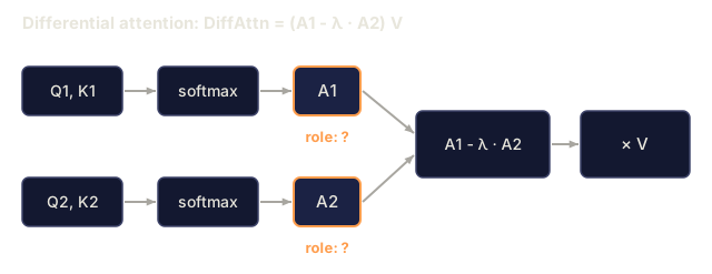
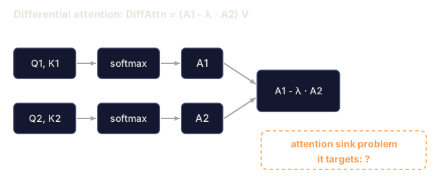
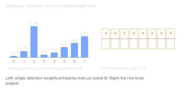
Differential attention computes two softmax attention maps from separate Q/K projections and subtracts a scaled copy of the second from the first. The goal is to cancel the attention sink.
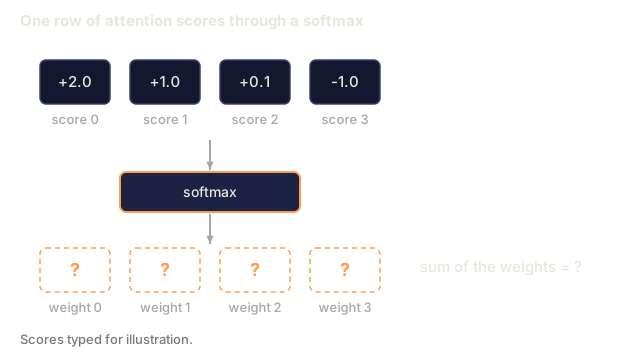
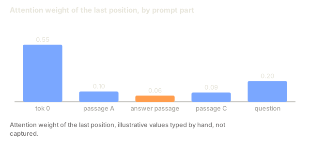
Regular attention has a sink problem. Softmax forces each row to sum to 1, so tokens that don't want to attend to anything in particular dump weight on the first token (or the first few). That steals capacity that should have gone to real content.
A1 = softmax(Q1 K1^T / √d)
A2 = softmax(Q2 K2^T / √d)
DiffAttn = (A1 - λ · A2) V
Here λ is a learned scalar (typically 0.5–0.8). A1 captures real content weights and A2 captures the sink, so subtracting cancels the sink and reallocates weight to relevant tokens.
Reported results (Microsoft 2024): 5–10% lower perplexity, 1.5–2× longer effective context at the same trained length, sharper needle-in-haystack retrieval.
Variant Comparison
| Variant | Compute | KV cache | Quality vs full | Production use |
|---|---|---|---|---|
| Full attention | O(N²) | O(N) per layer | baseline | every model's default layer |
| SWA (window 1024) | O(N·W) | O(W) per layer | -0.1 ppl, good with global layers | Gemma 2/3, Phi-3-Long |
| Local + strided sparse | O(N·√N) | mixed | similar to SWA | OpenAI sparse transformer, Longformer |
| BigBird (local + global + random) | O(N) approx | mixed | matches full at 2× context | early long-context BERT |
| Native Sparse (DeepSeek-V3.2) | O(N · active fraction) | O(N) | within 0.05 ppl | DeepSeek-V3.2, 2025 |
| Differential | O(2·N²) | O(2N) | -5 to -10% ppl | DIFF Transformer, early 2026 models |
Build It
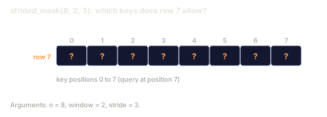
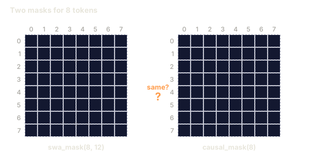
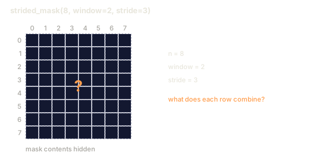
The code is in main.py, a standalone Python script that uses only the standard library. It renders full, SWA, and local+strided masks on an 8-token sequence (strided uses window=2, stride=3), runs a single-row differential attention demo, and prints KV cache sizes.
Step 1: full causal mask (baseline)
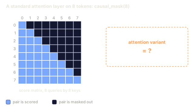
def causal_mask(n):
    return [[0.0 if j <= i else float("-inf") for j in range(n)] for i in range(n)]
This is the baseline: lower triangular, with zero weight above the diagonal.
Step 2: sliding window causal mask
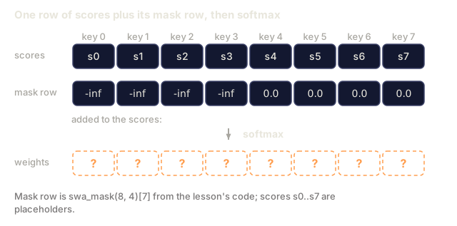
def swa_mask(n, window):
    M = [[float("-inf")] * n for _ in range(n)]
    for i in range(n):
        lo = max(0, i - window + 1)
        for j in range(lo, i + 1):
            M[i][j] = 0.0
    return M
One parameter: window. For window >= n, you recover full causal attention. For window = 1, each token attends just to itself.
Step 3: local + strided sparse mask
def strided_mask(n, window, stride):
    M = [[float("-inf")] * n for _ in range(n)]
    for i in range(n):
        lo = max(0, i - window + 1)
        for j in range(lo, i + 1):
            M[i][j] = 0.0
        for j in range(0, i + 1, stride):
            M[i][j] = 0.0
    return M
A dense local window plus each stride-th token back to the start of the sequence. main.py renders this pattern with window=2, stride=3 on 8 tokens. (Prose claim, not computed in main.py: the receptive field grows in log steps as you add layers.)
Step 4: differential attention
def diff_attention_row(q1, q2, K1, K2, V, mask_row, lam):
    _, w1 = attention_row(q1, K1, V, mask_row)
    _, w2 = attention_row(q2, K2, V, mask_row)
    diff = [a - lam * b for a, b in zip(w1, w2)]
    d_v = len(V[0])
    out = [0.0] * d_v
    for w, v in zip(diff, V):
        for j in range(d_v):
            out[j] += w * v[j]
    return out, diff
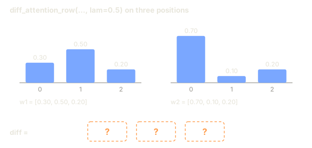
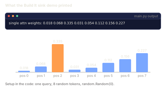
Two attention passes over one query row, subtracted with a mixing coefficient. The DIFF Transformer learns that coefficient; the script fixes lam=0.5 (Exercise 4 is the learned version). The demo runs one query against 8 random tokens, builds Q2 and K2 as small random perturbations of Q1 and K1, and prints the single-attention weights next to the differential ones. Because the data is random, no real sink shows up (the largest weight is at position 2), so this demo shows the arithmetic of the subtraction, not a collapsing sink. Differential weights can go negative.
Step 5: KV cache sizes
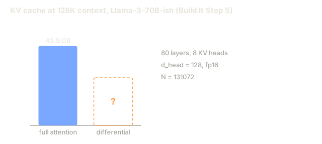
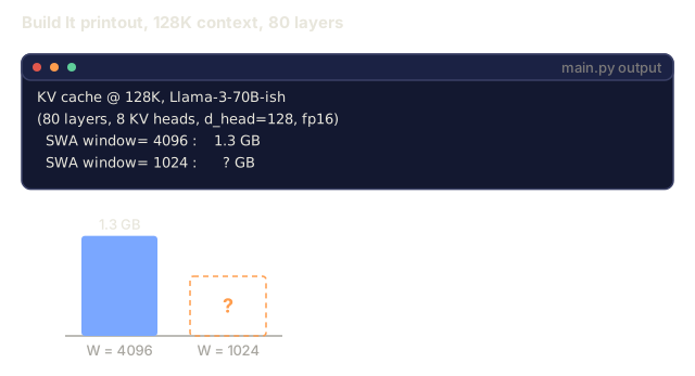
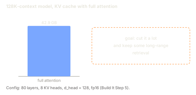
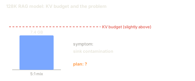
The script prints total KV cache across all 80 layers at N = 131072 for a Llama-3-70B-ish config (8 KV heads, d_head = 128, fp16). Full attention is 42.9 GB. Pure SWA drops to 1.3 GB at W = 4096 (32×) and 0.3 GB at W = 1024 (128×). The Gemma-3 mix (5:1, W = 1024) lands at 7.4 GB (5.8×), because the one global layer in six still caches the full 128K. Differential attention doubles full to 85.9 GB. There is no sparse or strided KV line in the script. Know what you're paying in memory before you pick one.
Use It
Two patterns from 2026 production code. The first is a model that mixes layer types:
from transformers import AutoModelForCausalLM
# Gemma 3 mixes SWA (window=1024) and global layers at 5:1.
model = AutoModelForCausalLM.from_pretrained("google/gemma-3-27b-it")
# print(model.config.sliding_window, model.config.layer_types)
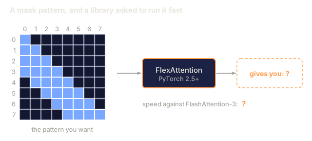
The second is FlexAttention in PyTorch 2.5+, which accepts a mask function:
from torch.nn.attention.flex_attention import flex_attention, create_block_mask

def swa_pattern(b, h, q_idx, kv_idx):
    return (q_idx - kv_idx < 1024) & (q_idx >= kv_idx)

mask = create_block_mask(swa_pattern, B=batch, H=heads, Q_LEN=n, KV_LEN=n)
out = flex_attention(q, k, v, block_mask=mask)
This compiles to a custom Triton kernel that runs within 10% of FlashAttention-3 speed for common patterns, and the mask function is a Python callable.
When to pick each:
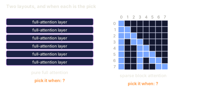
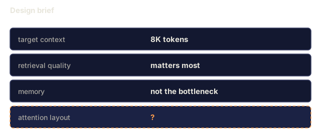
- Pure full attention. All layers up to ~16K context, or when retrieval quality matters most.
- SWA + global mix. Long context (>32K), where training and inference are memory-bound. This is the 2026 default above 32K.
- Sparse block attention. Custom kernel, custom pattern. Reserved for specialized workloads (retrieval, audio).
- Differential attention. Workloads where attention-sink contamination hurts, such as long-context RAG and needle-in-haystack retrieval.
Ship It
The skill in outputs/skill-attention-variant-picker.md picks an attention topology for a new model given target context length, retrieval demands, and training/inference compute profile.
I'd start from the SWA-plus-global mix for anything past 32K context, and I'd want a concrete reason before choosing pure full attention there. The comparison in main.py backs the memory side: at 128K it prints a 128× KV shrink for a pure 1024 window and a far smaller shrink for the 5:1 mix.
My bet is that the global layers are what you actually pay for. The gap between those two comes from the one global layer in six, which still caches the full 128K in that script's formula. I'd read that as the price of keeping long-range retrieval, and I'd tune the ratio before I touched the window size.
Differential attention is a bill you choose to pay. The script puts it at 2× the full-attention cache, and its sink demo is a single 8-token row with a fixed lam=0.5, so it shows the arithmetic of the subtraction and not a quality result. Before adopting it I'd run Exercise 4's retrieval task.
Exercises
- Easy. Run
main.py. Verify SWA atwindow=4zeroes everything outside the last 4 tokens per row. Verifywindow=nreproduces full causal attention bit-identically. - Medium. Implement causal SWA with
window=1024on top of the Lesson 14 capstone. Train for 1,000 steps on tinyshakespeare. How much does val loss regress vs full attention? How much does peak memory drop? - Hard. Implement a Gemma-3-style 5:1 layer mix (5 SWA, 1 global) in the capstone model. Compare loss, memory, and generation quality against pure-SWA and pure-global baselines at matched parameters.
- Hard. Implement differential attention with a learned
λper head. Train on a synthetic retrieval task (one needle, 2,000 distractors). Measure retrieval accuracy vs a single-attention baseline at matched parameters.
Key Terms
| Term | What people say | What it actually means |
|---|---|---|
| Sliding window attention (SWA) | "Local attention" | Each query attends to its last W tokens; KV cache shrinks to O(W). |
| Effective receptive field | "How far back the model sees" | In an L-layer SWA stack with window W, up to L × W tokens. |
| Longformer / BigBird | "Local + global + random" | Sparse patterns with a few always-attending global tokens; early long-context approach. |
| Native Sparse Attention | "DeepSeek's kernel trick" | Learn block-level sparsity; skip zero blocks at the kernel level while keeping quality. |
| Differential attention | "Two maps, one subtracts" | DIFF Transformer: subtract a learned λ times a second attention map from the first to cancel attention sinks. |
| Attention sink | "Weight bleeds to token 0" | Softmax normalization forces rows to sum to 1; uninformative queries dump weight on position 0. |
| FlexAttention | "Mask-as-Python" | PyTorch 2.5+ API that compiles arbitrary mask functions into FlashAttention-shape kernels. |
| Layer type mix | "5:1 SWA-to-global" | Interleave sparse and full attention layers in a stack to keep quality at lower memory. |
Further Reading
- Beltagy, Peters, Cohan (2020). Longformer: The Long-Document Transformer: the canonical sliding-window + global-token paper.
- Zaheer et al. (2020). Big Bird: Transformers for Longer Sequences: local + global + random.
- Child et al. (2019). Generating Long Sequences with Sparse Transformers: OpenAI's local+strided pattern.
- Gemma Team (2024). Gemma 2: Improving Open Language Models at a Practical Size: the 1:1 SWA:global mix.
- Gemma Team (2025). Gemma 3 technical report: the 5:1 mix with window=1024 that's now the textbook default.
- Ye et al. (2024). Differential Transformer: DIFF Transformer paper.
- Yuan et al. (2025). Native Sparse Attention: DeepSeek-V3.2's learned-sparsity attention.
- PyTorch: FlexAttention blog and docs: API reference for the mask-as-callable pattern in Use It.
Code
- main.py (python, 158 lines)