TAI BUI
Back to curriculum
BuildPython

GANs — Generator vs Discriminator

Goodfellow's trick in 2014 was to skip density entirely: two networks, one making fakes and one catching them, trained against each other until the fakes are indistinguishable from real. It shouldn't work, and it often doesn't. When it does, the samples are very sharp for narrow domains.

TIME: ~75 minutesPREREQUISITES: Phase 3 · 02 (Backprop), Phase 3 · 08 (Optimizers), Phase 8 · 02 (VAE)

Learning Objectives

  • Write the GAN minimax objective and explain what the generator and the discriminator each optimize.
  • Explain why the non-saturating generator loss gives G a usable gradient when D is confident.
  • Read the toy run's D(real), D(fake) and mode counts to spot a discriminator that is winning or a collapsing generator.
  • Match a failing GAN run to a likely cause and fix from the Pitfalls list.

The Problem

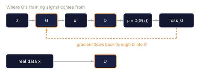
A generative adversarial network (GAN) trains two networks against each other. A classifier D(x) learns to tell real images from fakes, and a generator G(z) learns to fool D. The loss signal for G is whatever D currently thinks makes something look real. That signal shifts as G improves, so G chases a moving target. If both networks converge, G has learned the data distribution without anyone writing down log p(x).

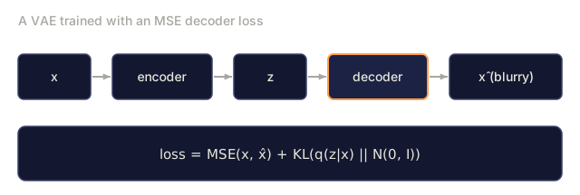
Here the starting point is the VAE's blur. A VAE's MSE decoder loss is Bayes-optimal for the mean image, and the mean of many plausible digits is a fuzzy digit. You want a loss that rewards plausibility instead of pixel-wise proximity to any one target. Plausibility has no closed form, so you learn it. Goodfellow's idea was to let the classifier be that learned loss.

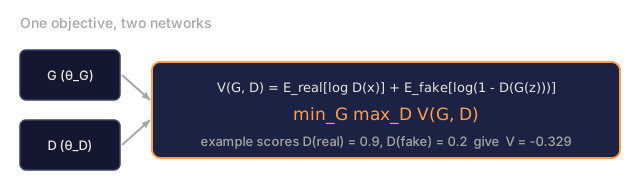
The math is a minimax game:

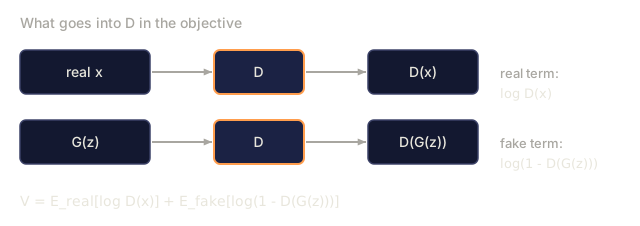
min_G max_D  E_real[log D(x)] + E_fake[log(1 - D(G(z)))]

In 2026 GANs are no longer the SOTA generator, since diffusion and flow matching took that crown. StyleGAN 2/3 still rank among the sharpest face models, though, GAN discriminators serve as perceptual losses in diffusion training, and adversarial training powers the fast 1-step distillations (SDXL-Turbo, SD3-Turbo, LCM) that let you ship real-time diffusion.
Warm-up0/3
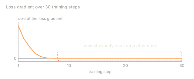
1. A model's loss gradient is almost exactly zero for many steps in a row. What happens to training?Warm-up
A line chart of the size of a loss gradient over 30 training steps. It falls from about 1 in the first steps and then lies on zero from step 8 to step 30, with that stretch boxed and labelled almost exactly zero, step after step.
Illustrative curve, not a measured run.
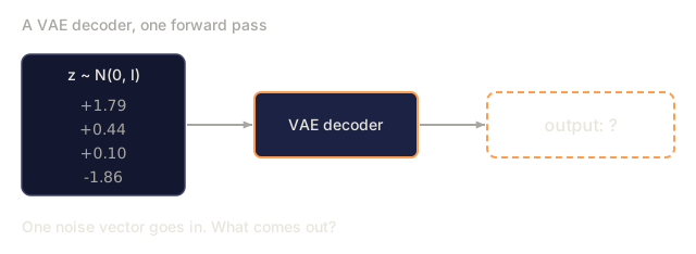
2. A VAE decoder takes a noise vector sampled from N(0, I). What does it output?Warm-up
A noise vector z drawn from N(0, I) with four example numbers is passed into a box labelled VAE decoder, which points to a dashed box labelled output with a question mark.
The four numbers are one random draw (numpy seed 3).
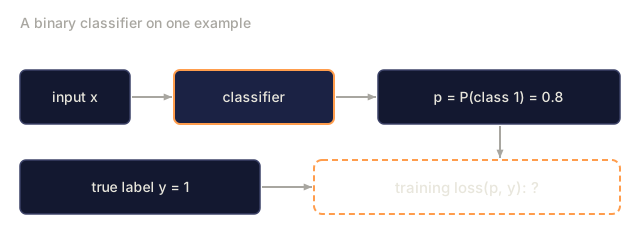
3. A binary classifier outputs a probability that an input belongs to class 1. Which loss is the standard choice for training it?Warm-up
An input x goes into a box labelled classifier, which outputs p equal to the probability of class 1, 0.8. Next to the true label y equal to 1, p feeds a dashed box asking for the training loss of p and y.
p = 0.8 is a typed example value.
Check: The Problem0/4
1. What does 'minimax' mean in the GAN objective min_G max_D?Define
Two boxes, G with weights theta_G and D with weights theta_D, both feed one highlighted box holding the objective V(G, D) as an expected log D(x) over real data plus an expected log of one minus D(G(z)) over fakes, with min over G of max over D of V written under it and an example value V equal to -0.329 for scores 0.9 and 0.2.
The example scores are typed; V is computed from them with natural logs.
2. A VAE with an MSE decoder loss tends to produce blurry samples. What is the best explanation?Explain
A VAE drawn as a chain: input x, encoder, latent z, decoder (highlighted), and a blurry output x-hat, with the training loss written below as MSE between x and x-hat plus a KL term to N(0, I).
3. Why is G described as chasing a moving target?Explain
A chain z, G, x-hat, D, p = D(G(z)), loss_G, with a dashed return path labelled gradient flows back through D into G, and a second input, real data x, also going into D.
4. In min_G max_D E_real[log D(x)] + E_fake[log(1 - D(G(z)))], what is D trying to do?Explain
Two paths into D: a real sample x gives D(x) and a generated sample G(z) gives D(G(z)); the real term log D(x) and the fake term log(1 - D(G(z))) are labelled, and the full objective V is written underneath.

The Concept

GAN training: generator and discriminator in minimax

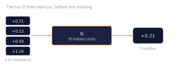
Generator G(z) maps a noise vector z ~ N(0, I) to a sample x̂. It's a decoder-shaped network (dense layers in the toy script, transposed convs in DCGAN-style image models).

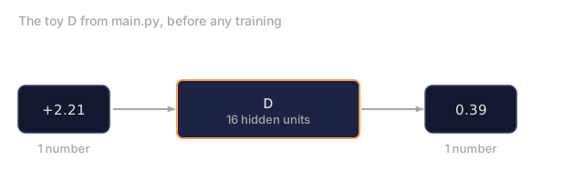
Discriminator D(x) maps a sample to a scalar probability (or score). Real should score 1, fake 0.

Loss. Two alternating updates:

  • Train D: loss_D = -[ log D(x) + log(1 - D(G(z))) ]. Binary cross-entropy with real=1 and fake=0.
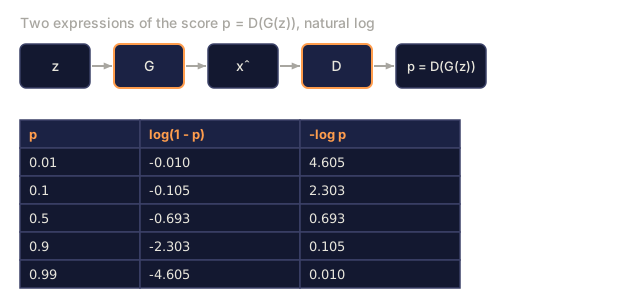
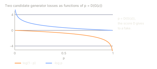
  • Train G: loss_G = -log D(G(z)). This is the non-saturating form Goodfellow used. The original log(1 - D(G(z))) saturates and kills gradients when D is confident.

Training loop. One step of D, then one step of G, repeated.

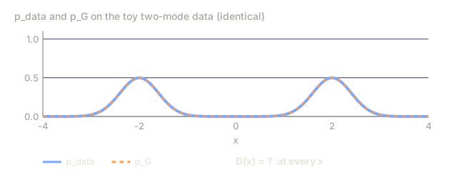
Why it works. If G perfectly matches p_data, D can't do better than chance and outputs 0.5 everywhere, and G gets no more gradient. That's the equilibrium.

Why it breaks. Mode collapse: G finds one mode D can't classify and keeps producing it. Vanishing gradient: D learns too fast and log D saturates. Training instability: small changes to learning rates or batch sizes can tip the whole run.
Check: The Concept0/7
1. What is the generator in a GAN?Define
Four noise numbers (z, drawn from N(0, I)) enter a highlighted box G with 16 hidden units, and one number, +0.21, comes out the other side.
Real forward pass of the untrained G built by main.py (seed 1).
2. What is the discriminator in a GAN?Define
One input number, +2.21, enters a highlighted box D with 16 hidden units, and one output number, 0.39, comes out.
Real forward pass of the untrained D built by main.py (seed 1), fed one sample from the real two-mode data.
3. What is the non-saturating loss for the generator?Define
A row z, G, x-hat, D, p = D(G(z)), and below it a table with p equal to 0.01, 0.1, 0.5, 0.9 and 0.99 and the two values log(1 - p) and negative log p for each: -0.010 and 4.605, -0.105 and 2.303, -0.693 and 0.693, -2.303 and 0.105, -4.605 and 0.010.
Both columns are computed from p; the table does not say which one a generator uses.
4. What is mode collapse?Define
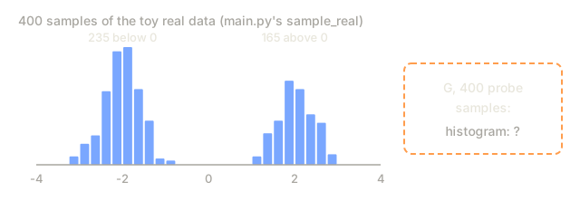
A histogram of 400 samples from the toy real data with two peaks, one near -2 (235 samples below 0) and one near 2 (165 above 0), next to a dashed box asking for the histogram of 400 samples from G.
Real draw from the lesson's sample_real: two Gaussians at -2 and +2, standard deviation 0.4.
5. What happens at equilibrium when G perfectly matches p_data?Explain
Two curves over x from -4 to 4, p_data as a solid blue line and p_G as a dashed orange line lying exactly on top of it, both with two peaks at -2 and 2, and a label asking for the value of D(x) at every x.
Densities of the Build It mixture (two Gaussians, standard deviation 0.4).
6. Why does the generator use the loss -log D(G(z)) instead of log(1 - D(G(z)))?Explain
Two curves against p from 0 to 1: log(1 - p) in orange, falling from about 0 at p near 0 to -5 near 1, and negative log p in blue, falling from 5 near 0 to about 0 at p near 1.
Plotted on the natural log scale, clipped at p = 0.005 and 0.995.
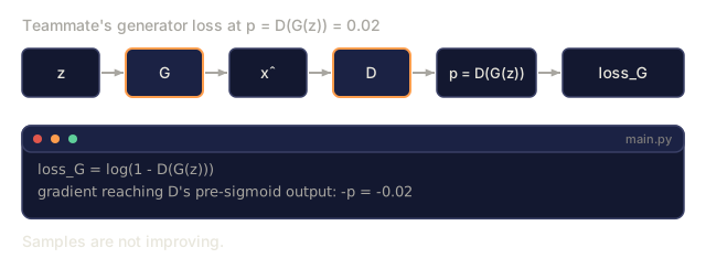
7. A teammate trains G with log(1 - D(G(z))). Early on D rejects every fake with high confidence and the samples do not improve. Which one-line change to G's loss fixes it?Analyze
A chain z, G, x-hat, D, p, loss_G, and below it the teammate's loss, log(1 - D(G(z))), with the gradient at p = 0.02 equal to minus p, minus 0.02, and a note that samples are not improving.
p = 0.02 is an illustrative value for a confident D.

Variants that made GANs work

YearInnovationFix
2015DCGANConv/deconv, batch norm, LeakyReLU, the first stable architecture.
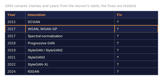
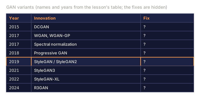
2017WGAN, WGAN-GPReplace BCE with Wasserstein distance + gradient penalty. Fixes vanishing gradient.
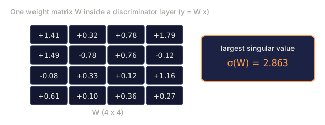
2017Spectral normalizationLipschitz-bound the discriminator. Still used in 2026 discriminators.
2018Progressive GANTrain low-res first, add layers. First megapixel results.
2019StyleGAN / StyleGAN2Mapping network + adaptive instance norm. State of the art for fixed-domain photorealism.
2021StyleGAN3Alias-free, translation-equivariant, still the face gold standard in 2026.
2022StyleGAN-XLConditional, class-aware, larger scale.
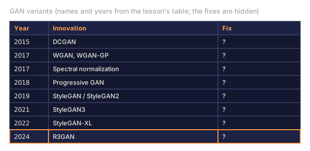
2024R3GANRebrands with stronger regularization; works on 1024² without tricks.
Check: Variants that made GANs work0/4
1. What problem do WGAN and WGAN-GP fix by replacing BCE with a Wasserstein distance plus a gradient penalty?Define
A table of GAN variants by year and innovation: DCGAN 2015, WGAN and WGAN-GP 2017, spectral normalization 2017, Progressive GAN 2018, StyleGAN and StyleGAN2 2019, StyleGAN3 2021, StyleGAN-XL 2022, R3GAN 2024. The Fix column holds a question mark in every row and the WGAN, WGAN-GP row is highlighted.
Year and innovation columns as in the lesson's variants table.
2. What is spectral normalization in a GAN?Define
A 4 by 4 matrix of weights W for one layer of a discriminator, with its largest singular value sigma(W) equal to 2.863 shown beside it.
Random matrix (numpy seed 0, scaled by 0.8) standing in for a D layer; sigma computed by SVD.
3. What is StyleGAN?Define
A table of GAN variants by year and innovation: DCGAN 2015, WGAN and WGAN-GP 2017, spectral normalization 2017, Progressive GAN 2018, StyleGAN and StyleGAN2 2019, StyleGAN3 2021, StyleGAN-XL 2022, R3GAN 2024. The Fix column holds a question mark in every row and the StyleGAN / StyleGAN2 row is highlighted.
Year and innovation columns as in the lesson's variants table.
4. What does R3GAN (2024) add that earlier variants needed tricks for?Define
A table of GAN variants by year and innovation: DCGAN 2015, WGAN and WGAN-GP 2017, spectral normalization 2017, Progressive GAN 2018, StyleGAN and StyleGAN2 2019, StyleGAN3 2021, StyleGAN-XL 2022, R3GAN 2024. The Fix column holds a question mark in every row and the R3GAN row is highlighted.
Year and innovation columns as in the lesson's variants table.

Build It

code/main.py trains a tiny GAN on 1-D data drawn from a mixture of two Gaussians. Generator and discriminator are single-hidden-layer MLPs, and the forward pass, backward pass, and minimax loop are all written by hand. Every 100 steps the script prints the mean D(real) and D(fake) plus how many probe samples land in each mode, and it flags mode collapse when one mode is starved. It does not log losses or detect vanishing gradients, so you infer that failure from D(real) and D(fake) staying pinned.

Step 1: non-saturating loss

The vanilla Goodfellow loss log(1 - D(G(z))) goes to 0 when D classifies G's fake as fake with high confidence. G's gradient is basically zero at that point, so G can't improve. The non-saturating form -log D(G(z)) has the opposite asymptote: it blows up when D is confident, which gives G a strong signal.

main.py never computes this loss as a function. Excerpted from update_g, it starts from the analytic gradient directly:

python
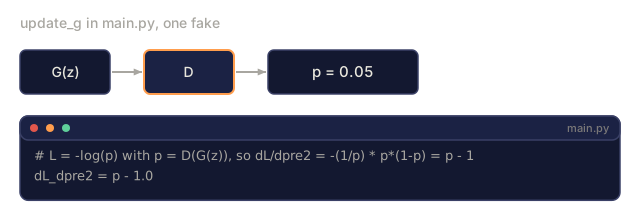
# L = -log(p) with p = D(G(z)), so dL/dpre2 = -(1/p) * p*(1-p) = p - 1
dL_dpre2 = p - 1.0

When D is confident the fake is fake, p is near 0 and this gradient is near -1, a strong push on G.

Step 2: one discriminator step per generator step

python
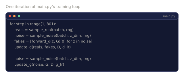
for step in range(1, 801):
    # train D
    reals = sample_real(batch, rng)
    noise = sample_noise(batch, z_dim, rng)
    fakes = [forward_g(z, G)[0] for z in noise]
    update_d(reals, fakes, D, d_lr)
 
    # train G
    noise = sample_noise(batch, z_dim, rng)  # fresh noise
    update_g(noise, G, D, g_lr)

update_g takes fresh noise and reruns G's forward pass itself, so its gradients are never stale.

Step 3: watch for mode collapse

python
if step % 100 == 0:
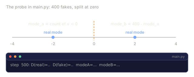
    probe_fakes = [forward_g(z, G)[0][0] for z in sample_noise(400, z_dim, rng)]
    mode_a = sum(1 for v in probe_fakes if v < 0)
    mode_b = 400 - mode_a
    if min(mode_a, mode_b) < 50:
        print("  [!] mode collapse")

The canonical symptom is that one of the two real modes stops being generated. The discriminator stops correcting it because it doesn't see that mode among the fakes.
Check: Build It0/8
1. In the Build It script, what makes it print the mode-collapse flag?Explain
A number line from -4 to 4 with the two real modes marked at -2 and 2 and a dashed split at 0; left of the split mode_a counts the probe values below 0, right of it mode_b is 400 minus mode_a. Below, the format of the line main.py prints every 100 steps, with the values left as dots.
The split and the print format come from Build It step 3; the dots stand for values.
2. Why does update_g sample fresh noise and rerun G's forward pass instead of reusing the fakes from the D step?Explain
The eight lines of main.py's training loop: sample reals, sample noise, build fakes with forward_g, update_d, then a second sample_noise call and update_g(noise, G, D, g_lr).
Excerpt of the lesson's Build It step 2, comments removed.
3. In update_g, dL_dpre2 = p - 1.0 where p = D(G(z)). If D scores a fake at p = 0.05, what is the gradient?Apply
A fake G(z) passes through D and gets the score p = 0.05; below, the two lines from update_g: the comment deriving dL/dpre2 as minus one over p times p(1 - p), and the statement dL_dpre2 = p - 1.0.
p = 0.05 is the stem's value; the code lines are quoted from main.py.
4. With the p - 1 gradient in update_g, which score for a fake gives G the strongest push?Apply
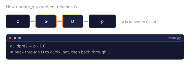
A chain z, G, D, p with a note that p is between 0 and 1, and below it the code line dL_dpre2 = p - 1.0 with a comment saying the gradient goes back through D to dL/dx_hat and then through G.
Structure from update_g in main.py.
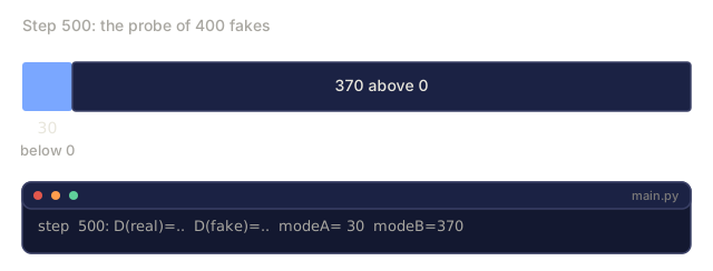
5. At step 500 the probe of 400 fakes puts 30 samples below zero and 370 above. What does the script do?Apply
A bar of 400 probe samples split into 30 below zero (a small blue segment) and 370 above zero, labelled step 500, and the format of the printed line for that step with modeA 30 and modeB 370.
Counts from the stem; D values left as dots.
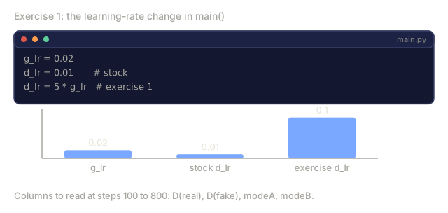
6. In exercise 1, d_lr is raised to 5 * g_lr. Which printed pattern shows D has taken over?Apply
The learning-rate lines of main(): g_lr 0.02, stock d_lr 0.01, and the exercise's d_lr set to 5 times g_lr, with a bar chart of g_lr 0.02, stock d_lr 0.01 and exercise d_lr 0.10, and a reminder of the columns printed every 100 steps.
Values from the lesson's exercise 1 and main().
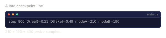
7. A late checkpoint prints D(real)=0.51, D(fake)=0.49 and mode counts of 210 and 190 out of 400. How do you read it?Apply
One line in the format main.py prints: D(real)=0.51, D(fake)=0.49, modeA=210, modeB=190, and a note that 210 plus 190 is 400 probe samples.
Typed from the stem; the step number is illustrative.
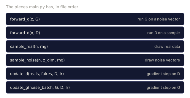
8. Which order matches one iteration of the training loop in main.py?Apply
A list of the six pieces of main.py in file order: forward_g, forward_d, sample_real, sample_noise, update_d and update_g, each with a short description.
Signatures from main.py; the list is in file order, not training order.

Pitfalls

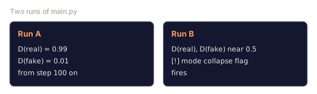
  • Discriminator too strong. Cut D's learning rate by 2-5x, or add instance/layer noise. If D(real) sits near 1 and D(fake) near 0 and stays there, G is dead.
  • Generator memorizes a mode. Add noise to D inputs, use a minibatch-discriminator layer, or switch to WGAN-GP.
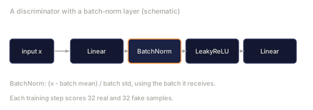
  • Batch norm leaking statistics. A real batch and a fake batch flowing through the same BN layer mix their statistics. Use instance norm or spectral norm instead (main.py has no norm layers, so you won't see this one in the toy run).
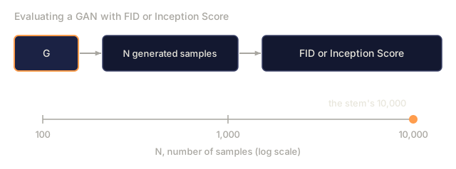
  • Inception-score gaming. FID and IS are noisy at low sample counts. Use at least 10k samples at eval.
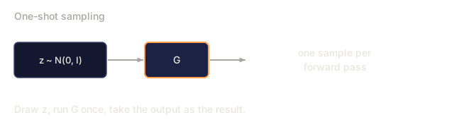
  • One-shot sampling is a lie for conditional tasks. You still need CFG scales, truncation tricks, and re-sampling to get usable outputs.
Check: Pitfalls0/5
1. Why does batch normalization cause problems in GAN training?Explain
A discriminator drawn as an input x followed by Linear, BatchNorm (highlighted), LeakyReLU and Linear boxes, with a note that BatchNorm subtracts the batch mean and divides by the batch std of the batch it receives, and a line saying each training step scores 32 real and 32 fake samples.
Schematic. The lesson's main.py has no norm layers.
2. Why should GAN evaluation use at least 10,000 samples?Explain
A pipeline G, N generated samples, FID or Inception Score, and below it a log-scale ruler of sample counts at 100, 1,000 and 10,000 with 10,000 marked.
3. For which kind of task is one-shot sampling misleading?Explain
A one-shot sampling pipeline: a noise vector z from N(0, I) goes through G in a single forward pass and gives one sample, with a line saying to draw z, run G once and take the output as the result.
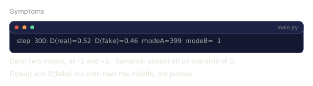
4. Samples show only one digit style although the data has several, and D(real) and D(fake) are not pinned. Which diagnosis and fix fit best?Analyze
A printed line from the stock run of main.py with D(real) 0.52, D(fake) 0.46, modeA 399 and modeB 1, with notes that the data has two modes at -2 and +2, almost all samples lie on one side of 0, and D(real) and D(fake) are near the middle.
Real line from main.py's stock run at step 300, the toy analogue of the stem (two modes instead of several digit styles).
5. Run A prints D(real)=0.99 and D(fake)=0.01 from step 100 on. Run B keeps D near 0.5 but the mode-collapse flag fires. Which run needs D's learning rate cut?Analyze
Two cards. Run A: D(real) = 0.99 and D(fake) = 0.01 from step 100 on. Run B: D(real) and D(fake) near 0.5, with the mode collapse flag firing.
Restates the stem.

Use It

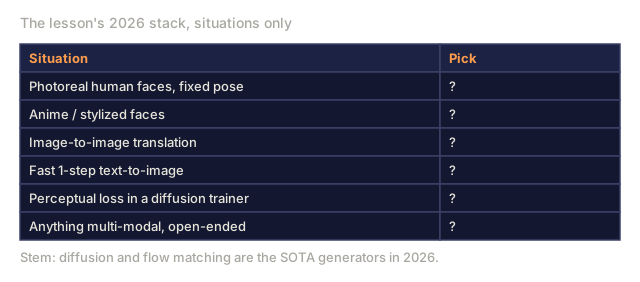
The 2026 GAN stack:

SituationPick
Photoreal human faces, fixed poseStyleGAN3 (sharpest, smallest)
Anime / stylized facesStyleGAN-XL or Stable Diffusion LoRA
Image-to-image translationPix2Pix / CycleGAN (Phase 8 · 04) or ControlNet (Phase 8 · 08)
Fast 1-step text-to-imageAdversarial distillation of diffusion (SDXL-Turbo, SD3-Turbo)
Perceptual loss inside a diffusion trainerSmall GAN discriminator on image crops
Anything multi-modal, open-endedDon't. Use diffusion or flow matching

GANs are sharp but narrow. Once your domain opens up (photos, arbitrary text prompts, video), switch to diffusion. The adversarial trick survives as a component (perceptual losses, distillation), not as a standalone generator.
Check: Use It0/4
1. Why do GANs still appear in 2026 stacks even though diffusion and flow matching are the SOTA generators?Explain
A two-column table of six situations from the lesson's Use It section (photoreal faces, anime faces, image-to-image translation, fast 1-step text-to-image, perceptual loss inside a diffusion trainer, anything multi-modal and open-ended) with a question mark in every Pick cell, and a line noting diffusion and flow matching are the SOTA generators in 2026.
Situation column quoted (shortened) from the lesson's table.
2. Which model is the best fit for photoreal human faces in a fixed pose?Apply
A task card with four rows: subject human faces, look photoreal, pose fixed, goal the sharpest result.
Restates the stem; no candidate is marked.
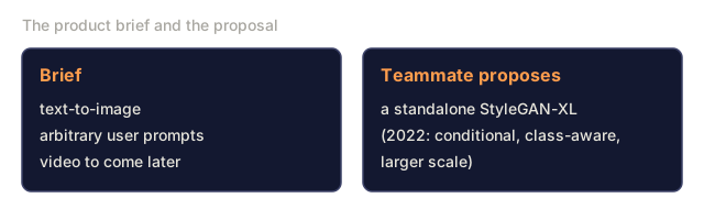
3. You must ship text-to-image for arbitrary user prompts and later add video. A teammate proposes a standalone StyleGAN-XL. What do you recommend?Design
Two cards: the brief, text-to-image for arbitrary user prompts with video to come later, and the teammate's proposal, a standalone StyleGAN-XL described in the lesson's table as conditional, class-aware and larger scale.
Brief from the stem; StyleGAN-XL description from the lesson's variants table.
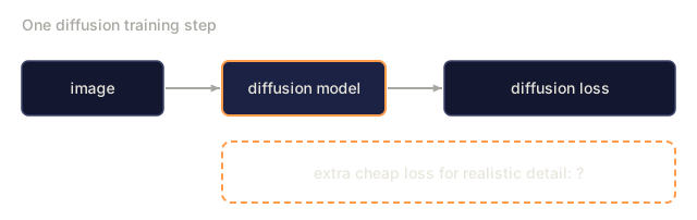
4. You train a diffusion model and want a cheap extra loss that rewards realistic detail. Which design fits?Design
A diffusion training step drawn as an image going into a highlighted diffusion model that feeds a diffusion loss, with a dashed box underneath for an extra cheap loss that rewards realistic detail, left as a question mark.

Ship It

Save outputs/skill-gan-debugger.md. The skill takes a failing GAN run (loss curves, sample grid, dataset size) and outputs a ranked list of likely causes, one-line fixes, and a rerun protocol.

Author's Note

I'd run main.py once with the stock settings and read the D(real) and D(fake) columns before looking at the mode counts. Both are D's average output, printed every 100 steps over 800 steps, so you watch the contest instead of just the result. The [!] mode collapse flag fires when either mode drops below 50 of the 400 probe samples, and I'd treat it as a smoke alarm, not a diagnosis.

My bet is that exercise 1 teaches more than the stock run. The script starts with D's learning rate at half of G's (0.01 against 0.02), and the exercise tips that balance toward D. I'd want to see what that imbalance looks like in the printed columns before trusting the Pitfalls advice about cutting D's learning rate.

Keep in mind what the script leaves out. It has no batch norm, so that pitfall is something you read about here, not something main.py will show you, and the same goes for spectral norm. What it does give you is the non-saturating gradient written out by hand, p - 1 flowing back through D and then through G, and I'd read that function before reaching for any variant in the table.

Exercises

  1. Easy. Run code/main.py with the stock settings. Then in main() change d_lr from 0.01 to 5 * g_lr and rerun. Watch D(real), D(fake) and the mode counts: does D(fake) get pinned near 0, and how quickly?
  2. Medium. Replace the Goodfellow BCE loss with the WGAN loss: loss_D = E[D(fake)] - E[D(real)], loss_G = -E[D(fake)], and clip D's weights to [-0.01, 0.01]. Is training more stable? Compare wall-clock convergence.
  3. Hard. Extend the 1-D example to 2-D data (mixture of 8 Gaussians on a ring). Track how many of the 8 modes the generator captures at steps 1k, 5k, 10k. Implement minibatch discrimination and re-measure.

Key Terms

TermWhat people sayWhat it actually means
Generator"G"Noise-to-sample network, G: z → x̂.
Discriminator"D"Classifier D: x → [0, 1], real vs fake.
Minimax"The game"min_G max_D of a joint objective.
Non-saturating loss"The fix"Use -log D(G(z)) for G instead of log(1 - D(G(z))).
Mode collapse"G memorized one thing"Generator produces few distinct outputs despite diverse data.
WGAN"Wasserstein"Replace BCE with Earth-Mover distance + gradient penalty; smoother gradient.
Spectral norm"Lipschitz trick"Constrain D's weight norms to bound its slope; stabilizes training.
StyleGAN"The one that works"Mapping network + AdaIN; best-in-class for faces, still in 2026.

Production note: one-shot inference is GAN's lasting advantage

GANs no longer win on sample quality for open-domain generation, but they still win on inference cost. In production-inference terms, a GAN has:

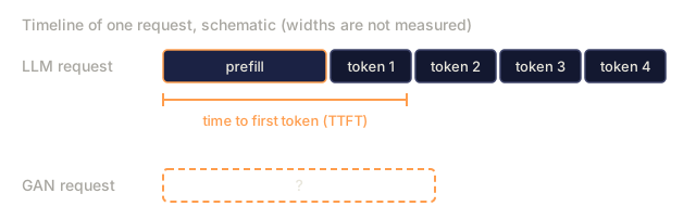
  • No prefill and decode stages. Generation is a single G(z) forward pass, so TTFT ≈ total latency.
  • No KV-cache pressure. The only state is the weights. Batch size is bounded by activation memory, not cache.
  • Trivial continuous batching. Each request takes the same fixed FLOPs, so a static batch at the server's target occupancy is usually optimal. No in-flight scheduler needed.

That's why GAN distillation (SDXL-Turbo, SD3-Turbo, ADD, LCM) is the dominant technique for fast text-to-image in 2026: it collapses a 20-50-step diffusion pipeline into 1-4 GAN-style forward passes while keeping the distribution of a diffusion base. The adversarial loss survives as a training-time knob for turning slow generators into fast ones.
Check: Production note: one-shot inference is GAN's lasting advantage0/2
1. Why is a GAN's time to first token roughly equal to its total latency?Explain
A schematic timeline of an LLM request with a prefill block and four token blocks and a bracket marking time to first token over the prefill and first token, and below it a dashed empty bar for a GAN request marked with a question mark.
Schematic of the LLM case; not measured.
2. Your product needs near-real-time text-to-image from a 30-step diffusion model. Which approach does the Production note point to?Design
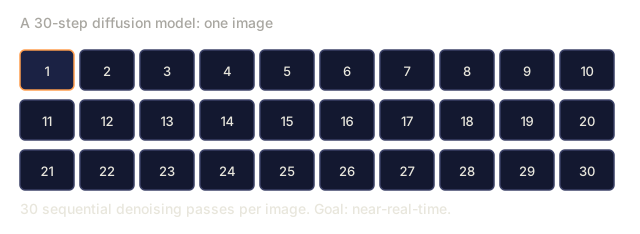
Thirty numbered boxes in three rows of ten, one per sampling step of a diffusion model, with a note that an image takes 30 sequential denoising passes and the goal is near-real-time.
Step count from the stem.

Further Reading

Code

Ships With