Autoencoders & Variational Autoencoders (VAE)
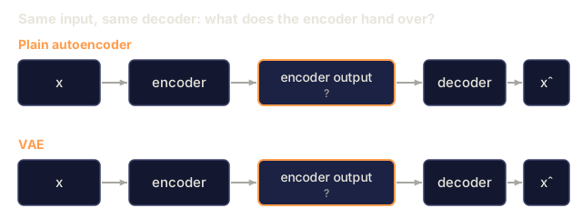
A plain autoencoder compresses, then reconstructs. It memorizes and does not generate. A VAE adds one trick: it forces the code to look Gaussian, and that gives you a sampler. The reparameterization `z = μ + σ·ε` is the reason the latent-diffusion and flow-matching image models you use in 2026 have a VAE at the input.
Learning Objectives
- Explain why a plain autoencoder cannot generate, and how a VAE's KL penalty toward N(0, I) turns the code space into something you can sample from.
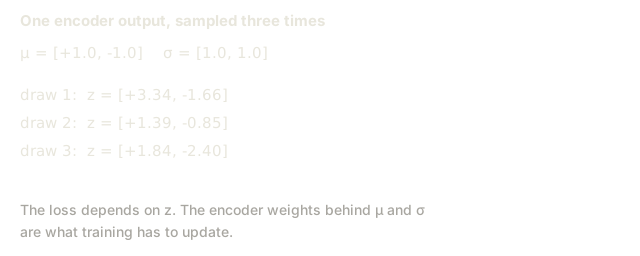
- Write the reparameterization z = μ + σ·ε and say why it lets gradients flow through a sampling step.
- Read the VAE loss (reconstruction + β·KL, with the closed-form Gaussian KL) and predict what raising or lowering β does to samples and the code space.
- Run the pure-Python VAE in main.py and map its forward, loss_value, backward and apply_update functions onto the lesson's math.
- Recognize posterior collapse and blurry samples, name the standard fixes, and place the VAE inside a latent-diffusion pipeline.
The Problem
An autoencoder compresses an input to a short code and reconstructs it from that code. A variational autoencoder (VAE) is an autoencoder whose encoder outputs a distribution over codes instead of a single code, with a penalty that pulls that distribution toward a Gaussian prior so you can sample from it.
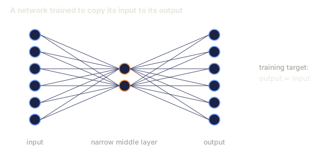
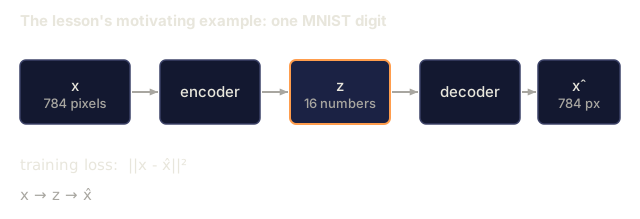
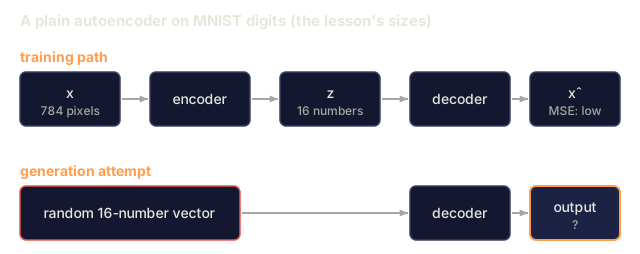
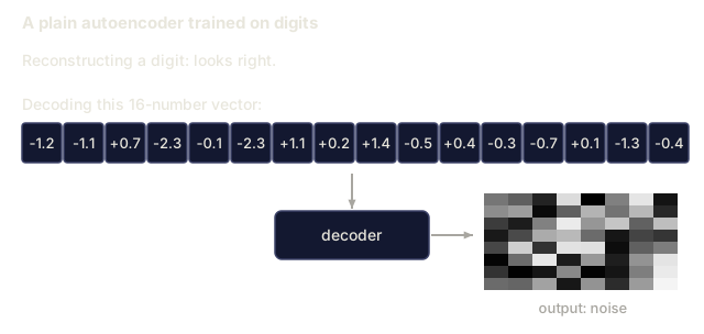
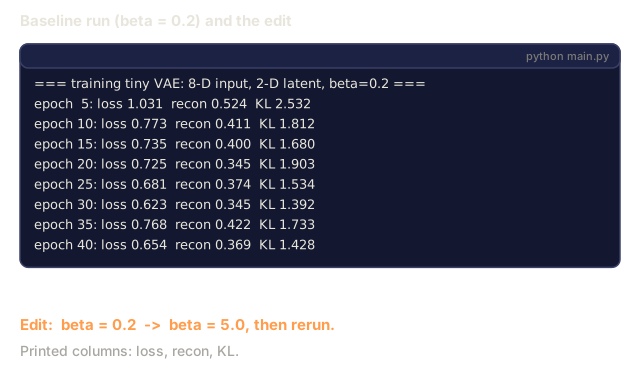
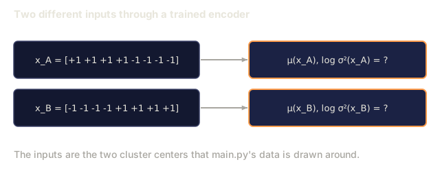
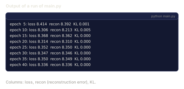
Start with the plain version. Compress a 784-pixel MNIST digit to a 16-number code, then reconstruct. (That is the motivating picture. The main.py you will run is a much smaller version: 8-D synthetic data from a two-cluster Gaussian mixture, a 2-D latent, a hidden layer of 10 units, 60 samples, 40 epochs, and β fixed at 0.2.) A plain autoencoder does well on reconstruction MSE, but the code space is lumpy. Pick a random point in it, decode it, and you get noise. There is no sampler here, just a compression model.
What you want is three things at once: (a) a code space that is a clean, smooth distribution you can sample from, say an isotropic Gaussian N(0, I), (b) decoded samples that look like plausible digits, and (c) an encoder and decoder that still compress well. Three goals, one architecture, one loss.
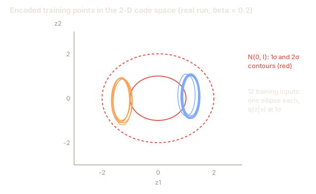
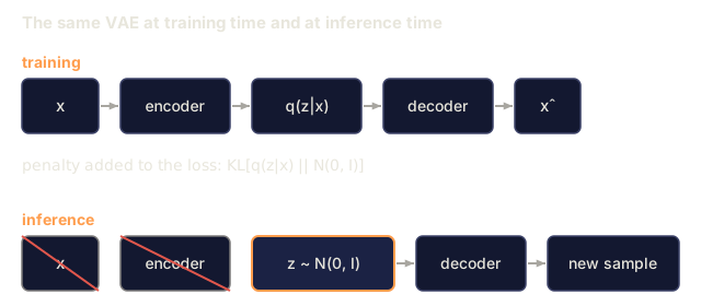
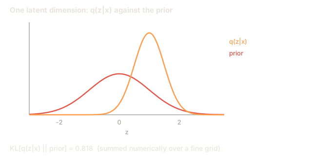
Kingma's 2013 VAE gets there by training the encoder to output a distribution q(z|x) = N(μ(x), σ(x)²), pulling it toward the prior N(0, I) with a KL penalty, and sampling z from q(z|x) before decoding. At inference time you drop the encoder, sample z ~ N(0, I), and decode. The KL penalty is what structures the code space.
In 2026 VAEs rarely ship standalone, since diffusion has outclassed them on raw image quality. They are the encoder of choice for latent-diffusion models (SD 1/2/XL/3, Flux, AudioCraft). Learn the VAE and you learn the invisible first layer of the image pipelines you use.
The Concept

Autoencoder. z = encoder(x), x̂ = decoder(z), loss = ||x - x̂||². The code space has no structure.
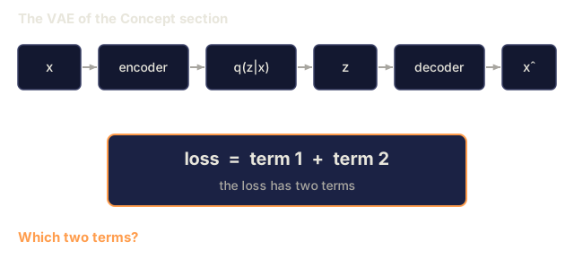
VAE encoder. Outputs two vectors, μ(x) and log σ²(x), which define q(z|x) = N(μ, diag(σ²)).
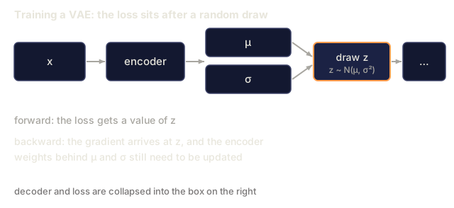
Reparameterization trick. Sampling from q(z|x) is not differentiable. Rewrite the sample as z = μ + σ·ε where ε ~ N(0, I). Now z is a deterministic function of (μ, σ) plus noise that has no parameters, so gradients flow through μ and σ.
Loss. The Evidence Lower BOund (ELBO) has two terms:
loss = reconstruction + β · KL[q(z|x) || N(0, I)]
     = ||x - x̂||²  + β · Σ_i ( σ_i² + μ_i² - log σ_i² - 1 ) / 2
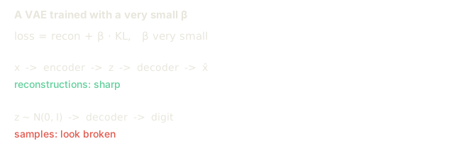
Reconstruction pushes x̂ toward x. KL pushes q(z|x) toward the prior. They trade off. Small β (<1) gives sharper samples and a code space that is less Gaussian. Large β (>1) gives a cleaner code space and blurrier samples. β-VAE (Higgins 2017) made this knob famous and kicked off disentanglement research.
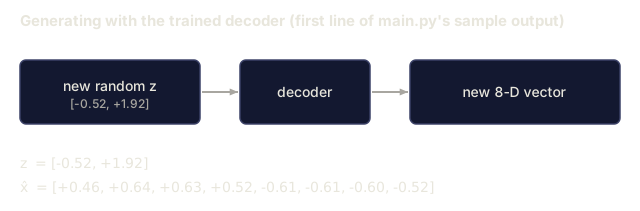
Sampling. At inference, draw z ~ N(0, I) and run it through the decoder. That is one forward pass, with no iterative sampling like diffusion.
Build It
code/main.py implements a tiny VAE without numpy or torch. Input is 8-dimensional synthetic data drawn from a 2-component Gaussian mixture in 8-D. Encoder and decoder are single hidden-layer MLPs. We implement tanh activation, forward pass, loss, and a hand-written backward pass. This is for teaching, not production.
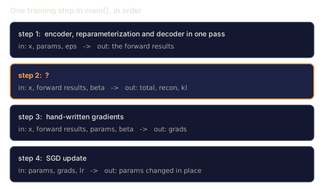
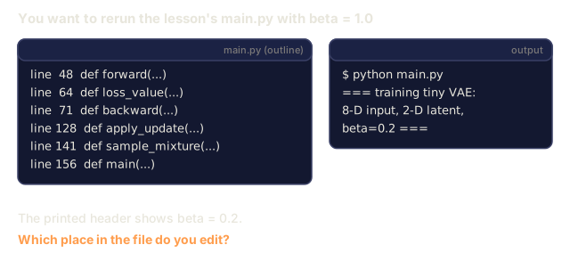
The snippets below are illustrative. main.py has no functions named encode, reparameterize, decode, elbo or sample. The real ones are forward (encoder, reparameterization and decoder in a single pass), loss_value (the ELBO), backward (hand-written gradients) and apply_update (the SGD step), and main() decodes its N(0, I) samples inline. The β in the file is a local variable, beta = 0.2, not a function argument.
Step 1: encoder forward
def encode(x, enc):
    h = tanh(add(matmul(enc["W1"], x), enc["b1"]))
    mu = add(matmul(enc["W_mu"], h), enc["b_mu"])
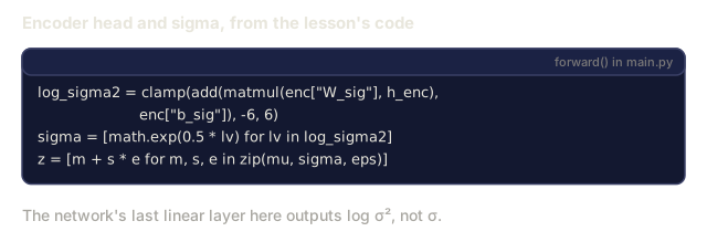
    log_sigma2 = add(matmul(enc["W_sig"], h), enc["b_sig"])
    return mu, log_sigma2
log σ² instead of σ so the network output is unconstrained (softplus of σ is a trap: gradients die at σ ≈ 0). The real forward also clamps log σ² to [-6, 6] to keep σ in a sane range; the snippet above leaves that out.
Step 2: reparameterize and decode
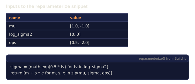
def reparameterize(mu, log_sigma2, rng):
    eps = [rng.gauss(0, 1) for _ in mu]
    sigma = [math.exp(0.5 * lv) for lv in log_sigma2]
    return [m + s * e for m, s, e in zip(mu, sigma, eps)]

def decode(z, dec):
    h = tanh(add(matmul(dec["W1"], z), dec["b1"]))
    return add(matmul(dec["W_out"], h), dec["b_out"])
Step 3: the ELBO
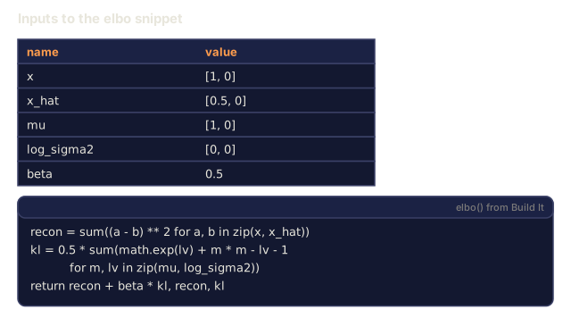
def elbo(x, x_hat, mu, log_sigma2, beta=1.0):
    recon = sum((a - b) ** 2 for a, b in zip(x, x_hat))
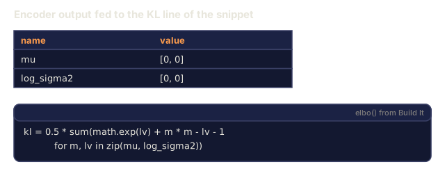
    kl = 0.5 * sum(math.exp(lv) + m * m - lv - 1 for m, lv in zip(mu, log_sigma2))
    return recon + beta * kl, recon, kl
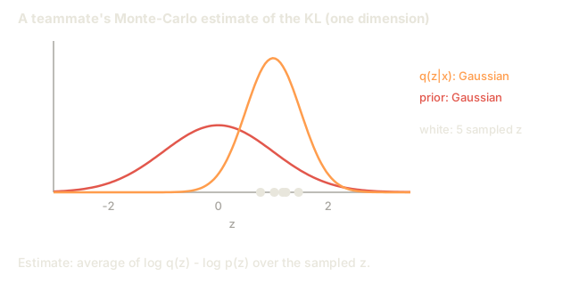
The KL has an exact closed form because both distributions are Gaussian, so there is no need to integrate numerically. People still ship code with Monte-Carlo KL estimates in 2026, and it is 3x slower for no reason. (That speed claim is prose only; main.py never compares the two estimators.)
Step 4: generate
def sample(dec, z_dim, rng):
    z = [rng.gauss(0, 1) for _ in range(z_dim)]
    return decode(z, dec)
That is the generative model: three lines. In main.py the same step runs inline in main(), which draws z from N(0, I) and pushes it through the decoder weights.
Pitfalls
- Posterior collapse. The KL term drives
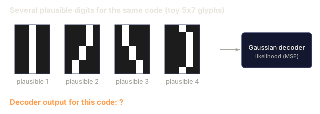
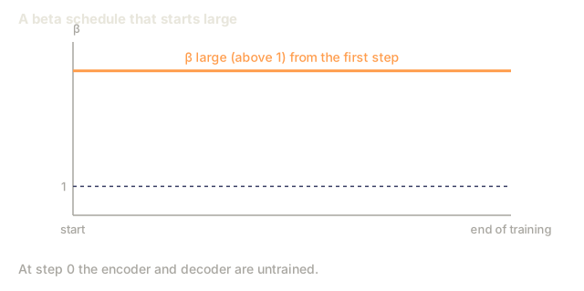
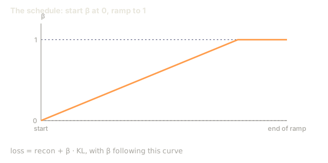
q(z|x) → N(0, I)so aggressively thatzcarries no info aboutx. Fix: β-annealing (start β=0, ramp to 1), free bits, or skip the KL on inactive dimensions. - Blurry samples. The Gaussian decoder likelihood implies MSE reconstruction, which is Bayes-optimal for L2 (the mean). The mean of a set of plausible digits is a fuzzy digit. Fix: discrete decoder (VQ-VAE, NVAE), or use the VAE as a compressor and run diffusion on its latents (this is what Stable Diffusion does).
- β too large, too early. See posterior collapse. Start at β≈0.01 and ramp.
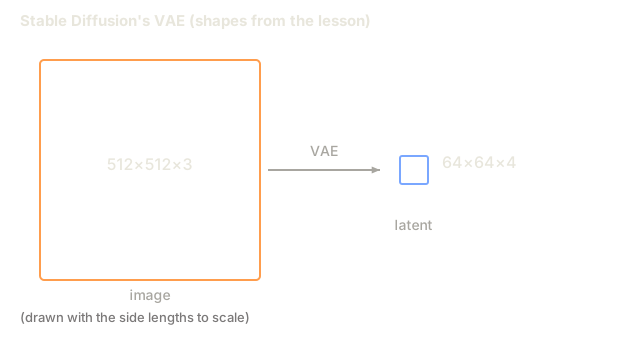
- Latent dim too small. 16-D works for MNIST, 256-D for ImageNet 256², 2048-D for ImageNet 1024². Stable Diffusion's VAE compresses 512×512×3 → 64×64×4 (each side shrinks 8x, so 64x in spatial area, while channels go from 3 to 4, which makes the total element count about 48x smaller).
The fixes above (β-annealing, free bits, skipping the KL on inactive dimensions) are prose only. main.py holds β fixed at 0.2 with no ramp, so none of them appear in the file.
Use It
The 2026 VAE stack:
| Situation | Pick |
|---|---|
| Image-latent encoder for diffusion | Stable Diffusion VAE (sd-vae-ft-ema) or Flux VAE |
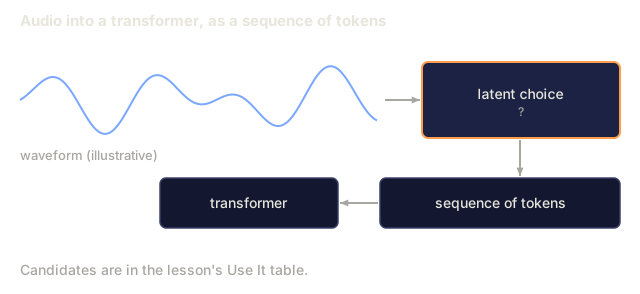
| Audio-latent encoder | Encodec (Meta), SoundStream, or DAC (Descript) |
| Video latents | Sora's spatiotemporal patches, Latte VAE, WAN VAE |
| Disentangled representation learning | β-VAE, FactorVAE, TCVAE |
| Discrete latents (for transformer modelling) | VQ-VAE, RVQ (ResidualVQ) |
| Continuous latents for generation | Plain VAE, then condition a flow/diffusion model in that latent space |
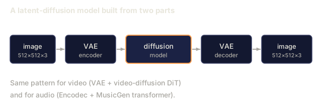
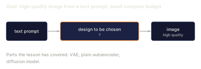
A latent-diffusion model is a VAE with a diffusion model living between encoder and decoder. The VAE does coarse compression, the diffusion model does the heavy lifting. Same pattern for video (VAE + video-diffusion DiT) and audio (Encodec + MusicGen transformer).
Ship It
Save outputs/skill-vae-trainer.md.
Skill takes: dataset profile + latent-dim target + downstream use (reconstruction, sampling, or latent-diffusion input) and outputs: architecture choice (plain/β/VQ/RVQ), β schedule, latent dim, decoder likelihood (Gaussian vs categorical), and evaluation plan (recon MSE, KL per dim, Fréchet distance between q(z|x) and N(0, I)).
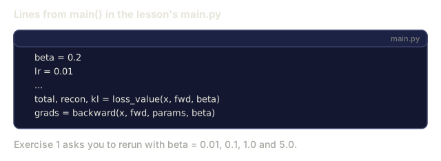
If I were working through the exercises, I'd start with the β sweep. The file trains with beta fixed at 0.2, and the balance between the reconstruction term and the KL term is set by that one number. Moving it and watching the printed recon and KL columns shows the balance directly, which the loss formula alone does not. With a large β, the KL column sinks toward zero, which is what the posterior collapse from Pitfalls looks like in a run.
My bet is that two choices here are worth copying into the VAEs you write later: the network predicts log σ² instead of σ, and the KL uses the closed-form Gaussian expression. Both are in the file in a few lines each.
I'd also keep the toy in proportion. The data is 8-D with two clusters and the latent is 2-D, so a decoder that turns N(0, I) samples into vectors near those clusters shows the sampler works. It does not show what a VAE does to MNIST digits, and the blur discussed in Pitfalls is something you have to go find with a larger model.
Exercises
- Easy. Edit the hardcoded
beta = 0.2line inmain()ofcode/main.pyand run it with0.01,0.1,1.0,5.0. Record the final reconstruction MSE and KL. Which β is Pareto-best for your synthetic data? - Medium. Replace the Gaussian decoder likelihood with a Bernoulli likelihood (cross-entropy loss). Compare sample quality on a binarized version of the same synthetic data.
- Hard. Extend
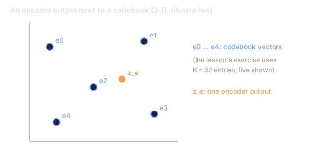
code/main.pyinto a mini VQ-VAE: replace the continuouszwith a nearest-neighbour lookup in a codebook of K=32 entries. Compare reconstruction MSE and report how many codebook entries get used (codebook collapse is real).
Key Terms
| Term | What people say | What it actually means |
|---|---|---|
| Autoencoder | Encode-decode network | x → z → x̂, learn MSE. Not generative. |
| VAE | AE with a sampler | Encoder outputs a distribution, KL penalty shapes code space. |
| ELBO | Evidence lower bound | log p(x) ≥ recon - KL[q(z|x) || p(z)]; tight when q = p(z|x). |
| Reparameterization | z = μ + σ·ε | Rewrites stochastic node as deterministic + pure noise. Enables backprop through sampling. |
| Prior | p(z) | Target distribution for the latent, typically N(0, I). |
| Posterior collapse | "KL term wins" | Encoder ignores x, outputs the prior; decoder must hallucinate. |
| β-VAE | Tunable KL weight | loss = recon + β·KL. Higher β = cleaner code space but blurrier samples (the knob behind disentanglement research). |
| VQ-VAE | Discrete latent | Replace continuous z with nearest codebook vector; enables transformer modelling. |
Production note: the VAE is the hottest path in a diffusion server
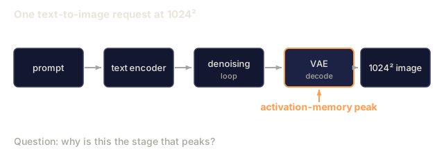
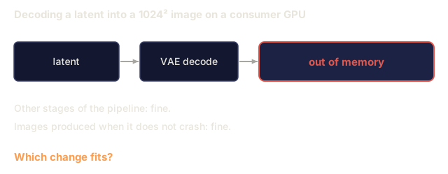
In a Stable Diffusion / Flux / SD3 pipeline the VAE is called twice per request: once to encode (if doing img2img / inpainting) and once to decode. At 1024² the decoder pass is often the single largest activation-memory peak in the whole pipeline because it upsamples 128×128×16 latents back to 1024×1024×3. Two practical consequences:
- Slice or tile the decode.
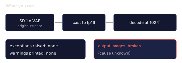
diffusersexposespipe.vae.enable_slicing()andpipe.vae.enable_tiling(). Tiling trades a small seam artifact forO(tile²)memory instead ofO(H·W). Tiling matters for 1024²+ on consumer GPUs. - bf16 decoder, fp32 numerics for the final resize. The SD 1.x VAE was released in fp32 and silently produces NaNs when cast to fp16 at 1024²+. SDXL ships
madebyollin/sdxl-vae-fp16-fix. Prefer the fp16-fix variant or use bf16.
Further Reading
- Kingma & Welling (2013). Auto-Encoding Variational Bayes: the VAE paper.
- Higgins et al. (2017). β-VAE: Learning Basic Visual Concepts with a Constrained Variational Framework: disentangled β-VAE.
- van den Oord et al. (2017). Neural Discrete Representation Learning: VQ-VAE.
- Vahdat & Kautz (2021). NVAE: A Deep Hierarchical Variational Autoencoder: state-of-the-art image VAE.
- Rombach et al. (2022). High-Resolution Image Synthesis with Latent Diffusion Models: Stable Diffusion; VAE as encoder.
- Défossez et al. (2022). High Fidelity Neural Audio Compression: Encodec, the audio VAE standard.
Code
- main.py (python, 202 lines)