LearnPython

Generative Models — Taxonomy & History

A generative model learns to sample from the distribution its training data came from, and the field sorts into five buckets by how each model gets there. Pick the wrong bucket and you will fight the math for weeks. Pick the right one and the last twelve years of progress stack cleanly in your head.

TIME: ~45 minutesPREREQUISITES: Phase 2 (ML Fundamentals), Phase 3 (Deep Learning Core), Phase 7 · 14 (Transformers)

Learning Objectives

Sort the five families of generative models by what each one models and how much of the density it exposes.
Explain the difference between explicit-density and implicit-density models, and which questions each can answer.
Place the major models from the 2013 VAE to 2026 one-step sampling in the right family and on the timeline.
Apply the five-question triage to a new paper and map a task to a family and its inference cost shape.

The Problem

A generative model learns to produce new samples from the same distribution as its training data: given samples drawn from some unknown p_data(x), it outputs new ones that look like they came from there. Faces, sentences, MIDI files, and protein structures look like the same problem if you squint.

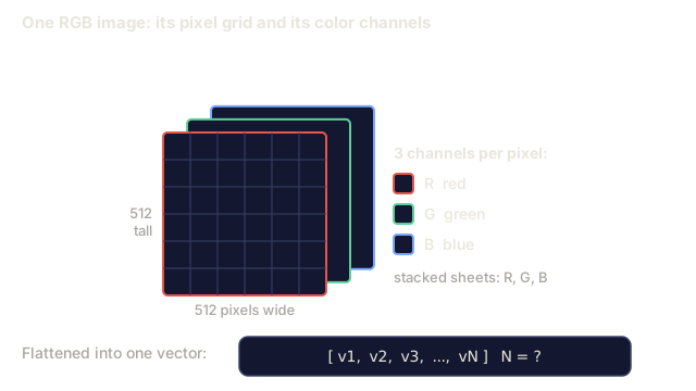
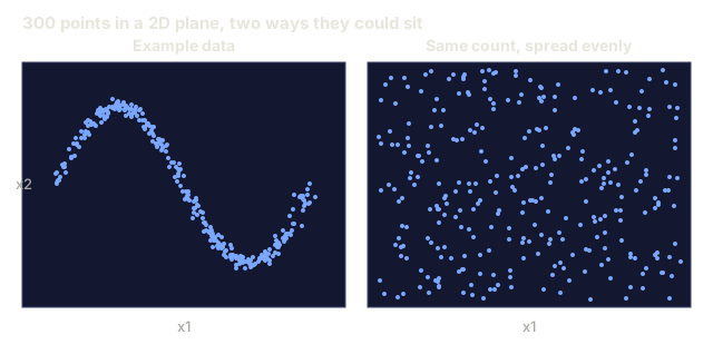
The rub is that p_data lives in a space with millions of dimensions (a 512x512 RGB image is ~786k dimensions), the samples sit on a thin manifold inside that space, and you have maybe 10M examples. Brute-forcing the density is hopeless, so generative models trade one hard problem for a slightly less hard one.

Five families have survived the last twelve years. Each makes a different compromise, and knowing which one tells you why it wins on some tasks and collapses on others.

Warm-up0/3

1. A 512x512 RGB image has three color channels per pixel. Flattened into one vector, about how many dimensions is that?Warm-up

Schematic, not to scale. N is what the question asks for.

2. An autoregressive Transformer like GPT predicts one token at a time. What does that imply for generating a long sequence?Warm-up

Illustrative tokens, typed.

3. A histogram of 2000 numbers has its bar heights scaled so the total area is 1. What does it approximate?Warm-up

Histogram of 2000 numbers spread from about -4 to 5.3 with two humps, bars 0.25 wide, vertical axis from 0 to 0.3, labelled total area of the bars equals 1. — Real samples from the lesson's main.py (seed 42). Bar height = count / (2000 x 0.25).

Check: The Problem0/3

1. The Key Terms table defines the manifold hypothesis as which of the following?Define

Two square scatter plots with 300 points each. The left plot shows points lying along a wavy curve. The right plot shows points spread evenly over the whole square. — Illustrative seeded points, not real data.

2. What is a generative model?Define

Real run of main.py, seed 42.

3. Why does every family settle for a compromise instead of modeling the full density of the data directly?Explain

Table of the five families and what each models in place of the full density: exact log p(x) with structure imposed, a lower bound, a sampler only, the score, a sequence of discrete tokens. — Summarized from The Concept section.

The Concept

Five families of generative models: taxonomy by what they model

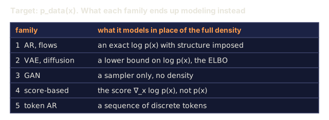
The five families differ in what they model and how much of the density they expose: the density itself, a bound on it, a sampler alone, the score, or a sequence of discrete tokens.

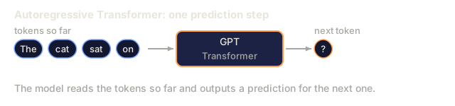
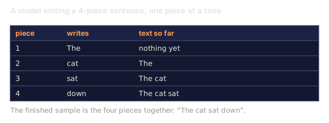
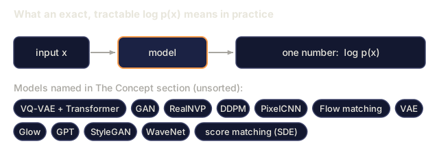
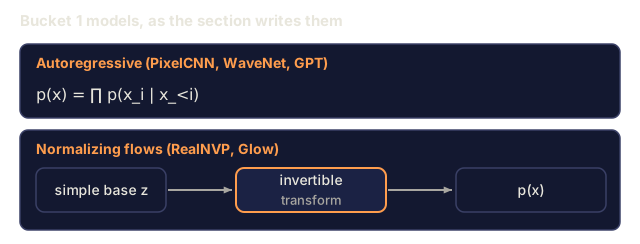
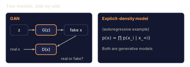
1. Explicit density, tractable. These models write log p(x) as a sum you can evaluate. Autoregressive models (PixelCNN, WaveNet, GPT) factorize p(x) = ∏ p(x_i | x_<i). Normalizing flows (RealNVP, Glow) build p(x) as an invertible transform of a simple base. The upside is exact likelihood and a clean training loss. The cost is that autoregressive inference is sequential (slow for long sequences) and flows need invertible architectures, which restricts the design.

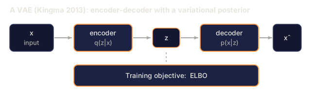
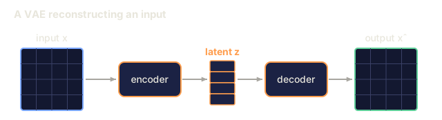
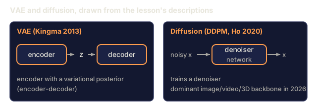
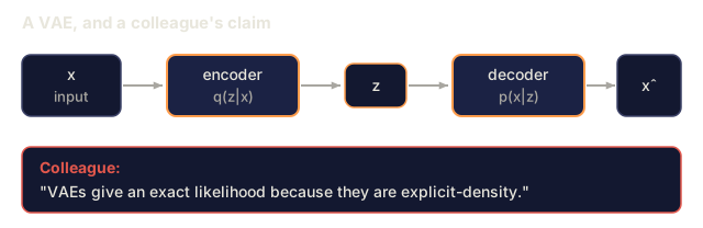
2. Explicit density, approximate. These models bound log p(x) from below (the ELBO) and optimize the bound. VAEs (Kingma 2013) use an encoder-decoder with a variational posterior. Diffusion models (DDPM, Ho 2020) train a denoiser that implicitly optimizes a weighted ELBO. Diffusion is the dominant image, video, and 3D backbone in 2026.

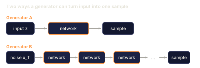
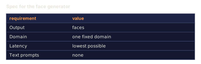
3. Implicit density. These models skip density entirely. A generator G(z) produces samples and a discriminator D(x) tells real from fake. GANs (Goodfellow 2014) are fast at inference (one forward pass) but notoriously unstable during training. StyleGAN 1/2/3 remain state of the art for fixed-domain photorealism (faces, bedrooms) even in 2026.

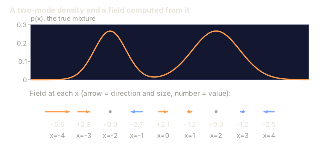
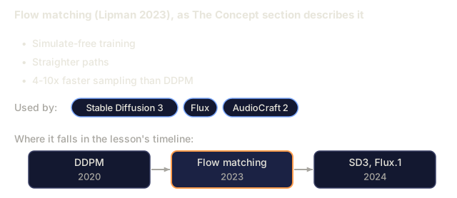
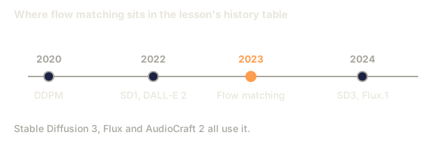
4. Score-based / continuous-time. These models learn the gradient of the log-density, ∇_x log p(x), called the score, directly. Song & Ermon (2019) showed score matching generalizes diffusion to an SDE. Flow matching (Lipman 2023) is the 2024-2026 favorite: simulate-free training, straighter paths, 4-10x faster sampling than DDPM. Stable Diffusion 3, Flux, and AudioCraft 2 all use flow matching.

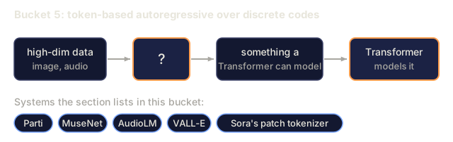
5. Token-based autoregressive over discrete codes. A VQ-VAE or residual quantizer compresses high-dim data into a short sequence of discrete tokens, then a Transformer models the token sequence. Parti, MuseNet, AudioLM, VALL-E, and Sora's patch tokenizer all use this. It is bucket 1 plus a learned tokenizer.

Check: The Concept0/15

1. According to the Key Terms table, how is ELBO defined?Define

Encoder-decoder diagram for a VAE: input x, encoder q(z|x), code z, decoder p(x|z), output x-hat, with a box underneath labelled training objective ELBO. — Schematic of the VAE named in the lesson's Concept section.

2. What does it mean for a model to have an explicit density?Define

Plot of a two-hump histogram of 2000 samples with a smooth kernel density curve drawn over it. — Real run of main.py, seed 42.

3. What is an implicit-density model?Define

A number line from -5 to 5 with ten points plotted, and below it terminal output listing ten generated sample values from -2.75 to +3.57. — Real run of main.py, seed 42 (excerpt).

4. In generative modeling, what is the score?Define

Curve of a two-hump density between -5 and 5, and underneath nine arrows at x from -4 to 4 pointing toward the nearer hump, each with a signed number. — Computed from the lesson's true mixture (0.4 N(-2, 0.6) + 0.6 N(2, 0.9)), not a trained model. Arrows are clipped at length 52 px for display; the numbers are exact.

5. What does autoregressive mean for a generative model?Define

Table with four rows for a four-piece sentence: columns piece, writes and text so far: The with nothing yet, cat after The, sat after The cat, down after The cat sat. — Illustrative sentence, typed.

6. What is a latent in a generative model?Define

A VAE schematic: a gridded input image, an encoder box, a small stack of four cells labelled latent z, a decoder box, and a gridded output image. — Schematic. Cell and grid counts are arbitrary.

7. Which families does The Concept section say give an exact, tractable log p(x)?Define

An input x goes into a model box that outputs one number log p(x). Below are twelve unsorted chips naming models from the lesson, such as PixelCNN, GAN, Glow, VAE and DDPM. — The chips are not grouped. Names come from The Concept section.

8. Where does The Concept section place flow matching in its five-family taxonomy?Define

Card listing flow matching facts: simulate-free training, straighter paths, 4-10 times faster sampling than DDPM, used by Stable Diffusion 3, Flux and AudioCraft 2, and a three-step timeline DDPM 2020, flow matching 2023, SD3 and Flux.1 2024. — Facts quoted from The Concept section and the history table.

9. How does bucket 5 (token-based autoregressive over discrete codes) turn high-dimensional data into something a Transformer can model?Explain

Pipeline from high-dim data through an unknown box marked question mark to something a Transformer can model, then a Transformer box, with chips for Parti, MuseNet, AudioLM, VALL-E and Sora's patch tokenizer. — The question-marked step is what the question asks about.

10. What trade-off does The Concept section name for bucket 1 models (autoregressive and normalizing flows)?Explain

Two cards. Autoregressive models with the formula p(x) equals the product of p(x_i given x_<i). Normalizing flows drawn as a simple base z, an invertible transform box, then p(x). — Both descriptions are from the lesson's Concept section.

11. Which question can an explicit-density model answer that a GAN cannot?Explain

Two panels. Left, a GAN: input z into generator G(z) producing a fake x, which with real x goes to discriminator D(x) deciding real or fake. Right, an autoregressive explicit-density model written as p(x) equals the product of p(x_i given x_<i). — Schematics based on The Concept section.

12. Why do VAEs and diffusion models share the explicit-density, approximate family?Explain

Two panels: a VAE drawn as an encoder, a latent z and a decoder in a row, and diffusion (DDPM) drawn as noisy x into a denoiser network box and out to x, each with the lesson's one-line description. — Schematic, from the lesson's Concept section.

13. Why is flow matching called the 2024-2026 favorite in the score-based family?Explain

Timeline with four marks: 2020 DDPM, 2022 SD1 and DALL-E 2, 2023 flow matching (highlighted), 2024 SD3 and Flux.1, with a note that Stable Diffusion 3, Flux and AudioCraft 2 use flow matching. — Years from the lesson's history table; spacing is schematic.

14. A colleague says VAEs give an exact likelihood because they are explicit-density. What is the flaw?Analyze

VAE diagram (input x, encoder, latent z, decoder, output x-hat) and a quote box with a colleague claiming VAEs give an exact likelihood because they are explicit-density. — The quote is the claim in the question.

15. A new paper's model draws each sample in one forward pass, never writes down log p(x), and reports unstable training. Which family does it resemble?Analyze

Five-row triage table. Density: never writes down log p(x). Sampling: one forward pass per sample. The other three rows are not stated. A note says training is reported as unstable. — Filled in from the facts in the question.

A brief history

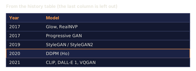
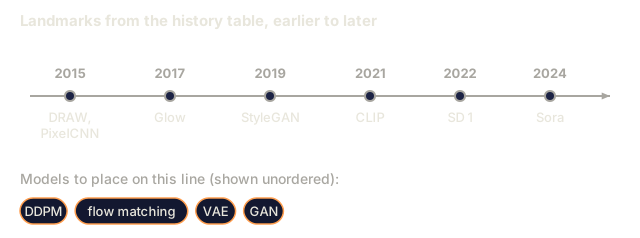
The table runs from the 2013 VAE to one-step sampling in 2026.

Year	Model	Why it mattered
2013	VAE (Kingma)	First deep generative model with a usable training loss.
2014	GAN (Goodfellow)	Implicit density, no likelihood, and shockingly sharp samples.
2015	DRAW, PixelCNN	Sequential image generation.
2017	Glow, RealNVP	Invertible flows; exact likelihood with depth.
2017	Progressive GAN	First megapixel faces.
2019	StyleGAN / StyleGAN2	Photorealistic faces still hard to beat for that one domain.
2020	DDPM (Ho)	Diffusion becomes practical.
2021	CLIP, DALL-E 1, VQGAN	Text-to-image goes mainstream.
2022	Imagen, Stable Diffusion 1, DALL-E 2	Latent diffusion + text conditioning = commodity.
2022	ControlNet, LoRA	Fine control over pretrained diffusion.
2023	SDXL, Midjourney v5, Flow matching	Scale + better training dynamics.
2024	Sora, Stable Diffusion 3, Flux.1	Video diffusion; flow matching wins.
2025	Veo 2, Kling 1.5, Runway Gen-3, Nano Banana	Production-grade video.
2026	Consistency + Rectified Flow	One-step sampling from diffusion backbones.

Check: A brief history0/2

1. According to the A brief history table, what does the 2020 entry credit DDPM with?Define

Table of five history rows with Year and Model columns only: 2017 Glow and RealNVP, 2017 Progressive GAN, 2019 StyleGAN, 2020 DDPM highlighted, 2021 CLIP, DALL-E 1 and VQGAN. — The 'Why it mattered' column is hidden on purpose.

2. Which order puts these four models on the timeline from earliest to latest?Define

Landmark years from the history table. The four chips are the models to be ordered.

The five-question triage

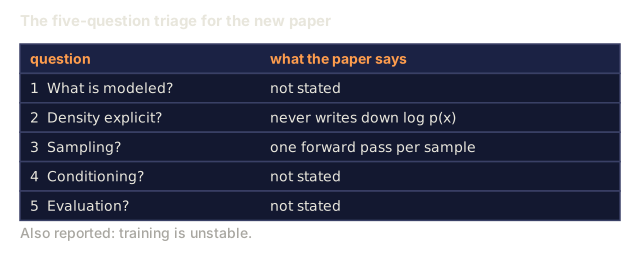
When a new generative model paper drops, answer these five questions before you read the method section.

What is being modeled? Pixels, latents, discrete tokens, 3D Gaussians, meshes, waveforms?
Is the density explicit or implicit? Do they write down log p(x)?
Sampling: one-shot or iterative? Iterative means slower inference; one-shot usually means adversarial or distilled.
Conditioning: unconditional, class, text, image, pose? This determines the loss and architecture scaffolding.
Evaluation: FID, CLIP score, IS, human preference, task accuracy? Each has known failure modes (see Lesson 14).

You will answer these five again in every lesson of this phase. By the end they will be reflex.

Check: The five-question triage0/1

1. In the five-question triage, which question tells you whether inference will be iterative and slow or one-shot?Define

Two generic generator diagrams. Generator A: an input z goes through one network box to a sample. Generator B: noise x_T goes through a chain of network boxes, then an ellipsis, to a sample. — Generic shapes for illustration, not a specific model.

Build It

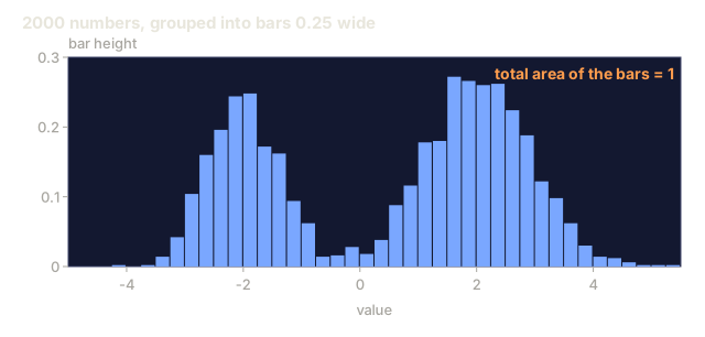
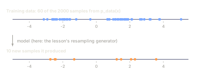
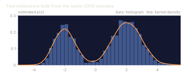
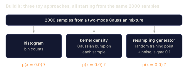
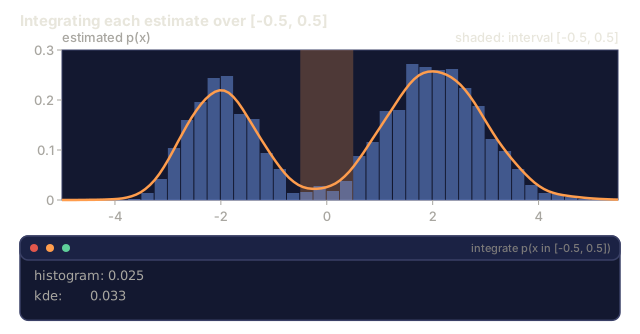
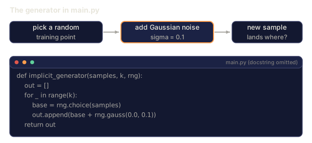
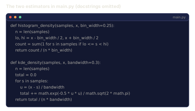
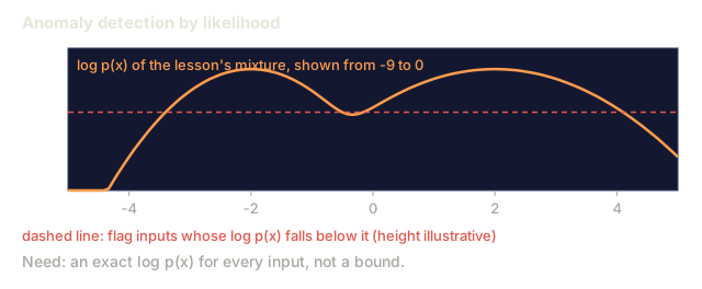
The code here is a small visualization. It draws 2000 samples from a known two-mode Gaussian mixture (modes at -2 with sigma 0.6 and +2 with sigma 0.9, weight 0.4 on the first) and runs three toy approaches on them, so you can see explicit vs implicit density on a problem that prints on one screen. A histogram and a Gaussian kernel density estimate (KDE) both estimate p(x) straight from the samples. Nothing is fitted as a mixture model. The third approach is an implicit generator that picks a random training point and adds Gaussian noise (sigma 0.1). It does no nearest-neighbour lookup.

Run main.py. It prints an ASCII histogram of the samples, evaluates p(x=0.0) three ways, integrates p(x in [-0.5, 0.5]) under the histogram and the KDE, and draws 10 new samples from the generator. The real output with seed 42:

=== 2000 samples from a two-mode Gaussian mixture ===
                          #             
                          ####          
           ##             ####          
           ##             #####         
          ###             ######        
         ######         ########        
         ######         ########        
         ######        ##########       
        ########       ###########      
        ########      ############      
        #########     #############     
       ##########  # ###############    
----------------------------------------
-5.0                                5.0

evaluate p(x=0.0) three ways:
  histogram density: 0.0180
  kernel density:    0.0258
  implicit generator: N/A (only samples, no density)

integrate p(x in [-0.5, 0.5]):
  histogram: 0.025
  kde:       0.033

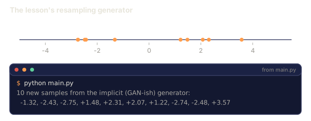
10 new samples from the implicit (GAN-ish) generator:
  -1.32, -2.43, -2.75, +1.48, +2.31, +2.07, +1.22, -2.74, -2.48, +3.57

takeaway: explicit density (buckets 1-2 in the doc) lets you answer
'how likely is this point?'. implicit (bucket 3) does not.

The histogram and KDE are non-parametric estimators, not the bucket 1 or 2 models themselves. The script's takeaway line says "buckets 1-2 in the doc" because both estimators expose a density the way those buckets do. Notice that the histogram and the KDE let you ask "how likely is this point?" and the generator cannot. That is the explicit vs implicit distinction, and it will keep coming up in the lessons ahead.

Check: Build It0/4

1. In Build It, which of the three toy approaches cannot answer 'how likely is this point?'Apply

One box of 2000 samples with three arrows to three boxes: histogram, kernel density, and resampling generator (random training point plus noise with sigma 0.1). Under each box is the question p of x equals 0.0 with a question mark. — Descriptions from the Build It section.

2. Build It integrates p(x) over [-0.5, 0.5] and prints 0.025 for the histogram and 0.033 for the KDE. What does this show?Apply

Plot of a two-hump histogram and kernel density curve with the interval from -0.5 to 0.5 shaded, and a terminal listing histogram 0.025 and kde 0.033. — Real run of main.py, seed 42.

3. The generator in main.py picks a random training point and adds Gaussian noise with sigma 0.1. Where is a new sample most likely to land?Apply

Three boxes: pick a random training point, add Gaussian noise with sigma 0.1, new sample lands where. Below is the source of implicit_generator from main.py. — Copied by the generator script from the lesson's main.py.

4. A teammate says the histogram and KDE in main.py are the bucket 1 and 2 models. What is wrong with that?Analyze

Source code of the histogram_density and kde_density functions from main.py, shown without docstrings. — Copied by the generator script from the lesson's main.py.

Use It

Which family fits which task in 2026?

Task	Best family	Why
Photoreal faces, narrow domain	StyleGAN 2/3	Still sharpest, fastest inference.
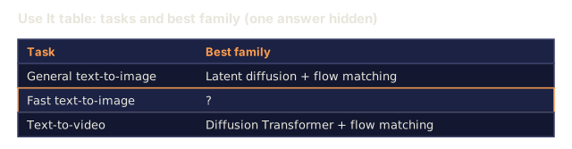
General text-to-image	Latent diffusion + flow matching	SD3, Flux.1, DALL-E 3.
Fast text-to-image	Rectified flow + distillation	SDXL-Turbo, SD3-Turbo, LCM.
Text-to-video	Diffusion Transformer + flow matching	Sora, Veo 2, Kling.
Speech + music	Token-based AR (AudioLM, VALL-E, MusicGen) or flow matching (AudioCraft 2)	Discrete tokens scale cheaply.
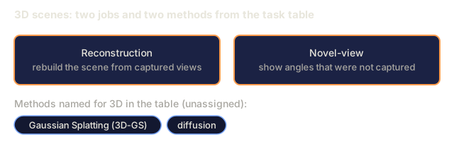
3D scenes	Gaussian Splatting fit, diffusion prior	3D-GS for reconstruction, diffusion for novel-view.
Density estimation (no sampling)	Flows	Exact `log p(x)` with one-pass sampling (autoregressive models are exact too, but sample sequentially).
Simulation / physics	Flow matching, score SDE	Straight-line paths, smooth vector fields.

Check: Use It0/4

1. For 3D scenes, which pairing does the task table give?Apply

Two task boxes, Reconstruction and Novel-view, and two unassigned method chips, Gaussian Splatting (3D-GS) and diffusion. — Task descriptions are plain-language glosses; the pairing is left open.

2. Per the Use It table, which family is recommended for fast text-to-image generation?Apply

Three-row task table with the fast text-to-image family hidden as a question mark; general text-to-image shows latent diffusion plus flow matching and text-to-video shows diffusion Transformer plus flow matching. — Rows quoted from the Use It table.

3. You must ship a face generator for one fixed domain with the lowest possible latency and no text prompts. Which family fits best?Design

A four-row requirement table: output is faces, domain is one fixed domain, latency is lowest possible, text prompts are none. — The requirements as stated in the question.

4. You are building anomaly detection that flags inputs with low likelihood under the model, and you want an exact log p(x), not a bound. Which family fits?Design

Plot of the log density of a two-hump mixture from -9 to 0 over x from -5 to 5, with a dashed horizontal threshold line, explained in a note underneath as the flagging level. — Curve computed from the lesson's mixture, clipped below -9 for display; threshold height is illustrative.

Ship It

Save as outputs/skill-model-chooser.md.

The skill takes a task description and outputs four things: which family to use, a ranked list of three open and three hosted options, the likely failure mode to watch for, and a compute/time budget.

Author's Note

I'd run the density question from the triage first on any new paper: does it expose p(x) or give you a sampler alone? main.py makes that concrete. The histogram and the KDE both return a number for p(x) at a query point and integrate it over [-0.5, 0.5], while the implicit generator prints samples and a line saying there is no density.

My bet is that the resampling generator deserves some suspicion. In main.py it picks a training point at random and adds noise with a standard deviation of 0.1, so each output is a training point plus a small jitter. There is no discriminator and no training loop. I'd read "GAN-ish" as a label for "no p(x)" and not as a picture of how a GAN learns.

I'd also check the production note's "fewer steps × same step cost" versus "same steps × cheaper step cost" split against numbers in the paper, because nothing in main.py runs a multi-step sampler and the script can't show you that cost curve.

Exercises

Easy. For each of these five products, identify the family and backbone: ChatGPT image, Midjourney v7, Sora, Runway Gen-3, ElevenLabs. Back each answer with a public technical report.
Medium. The paper you are about to read tomorrow claims 100x faster sampling than diffusion. Write down three questions to check whether the speedup survives conditioning and high resolution.
Hard. Take one domain you care about (e.g. protein structure, CAD, molecules, trajectories). Answer the five-question triage for the current SOTA model in that domain and sketch what a better model would change.

Key Terms

Term	What people say	What it actually means
Generative model	"It makes new stuff"	Learns a sampler for `p_data(x)`, optionally exposes `log p(x)`.
Explicit density	"You can evaluate it"	Model provides a closed-form or tractable `log p(x)`.
Implicit density	"GAN-style"	A sampler, with no way to evaluate `p(x)` of a given point.
ELBO	"Evidence lower bound"	A tractable lower bound on `log p(x)`; VAEs and diffusion optimize it.
Score	"Gradient of log-density"	`∇_x log p(x)`; diffusion and SDE models learn this field.
Manifold hypothesis	"Data lives on a surface"	High-dim data concentrates on a low-dim manifold; why dimensionality reduction works.
Autoregressive	"Predict the next piece"	Factorize joint as product of conditionals.
Latent	"Compressed code"	Low-dim representation from which a decoder can reconstruct the input.

Production note: five families, five inference shapes

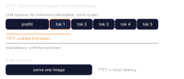
Each family maps to a different inference-server cost curve. Production-inference writing frames LLM inference as prefill plus decode, and the same decomposition applies here:

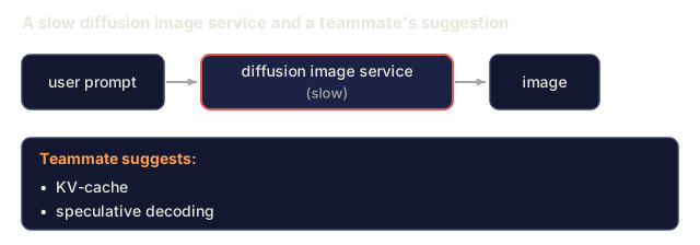
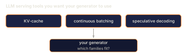
Autoregressive (bucket 1 and 5). Sequential decode dominates latency, and KV-cache, continuous batching, and speculative decoding all apply directly.
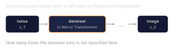
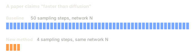
VAE / diffusion / flow-matching (buckets 2 and 4). There is no decode in the LLM sense. Cost = num_steps × step_cost, and step_cost is a transformer or U-Net forward at the full latent resolution. The production knobs are step count (DDIM / DPM-Solver / distillation), batch size, and precision (bf16 / fp8 / int4).
GAN (bucket 3). One forward pass, with no schedule and no KV-cache. TTFT ≈ total latency, which is why StyleGAN still wins on narrow-domain UX.

When you see "faster than diffusion" in a paper abstract, translate it to "fewer steps × same step cost" or "same steps × cheaper step cost". Anything beyond those two readings deserves a second look.

Check: Production note: five families, five inference shapes0/5

1. According to the production note, what determines the inference cost of a diffusion or flow-matching image model?Define

Pipeline: noise x_T, a denoiser network box labelled U-Net or Transformer, an ellipsis, then the image x_0, with a note that the number of denoiser runs is not specified. — Schematic only.

2. Why does the production note say a GAN's TTFT is roughly its total latency?Explain

Top row, an LLM request drawn as a prefill block then five token blocks with TTFT marked up to the first token and total latency marked to the last. Bottom row, a GAN request drawn as one block labelled serve one image, with TTFT approximately equal to total latency. — Illustrative layout, not measured times.

3. A diffusion image service is slow, and a teammate suggests KV-cache and speculative decoding. Why is that the wrong lever?Analyze

A service diagram: user prompt, a diffusion image service marked slow, and the image. Below it a box listing the teammate's suggestions: KV-cache and speculative decoding. — Schematic of the situation in the question.

4. A paper claims 'faster than diffusion', and its method runs 4 sampling steps with the same network as a baseline that runs 50. Which reading from the production note applies?Analyze

Two rows of step blocks: the baseline with 50 blocks and the new method with 4 blocks, both labelled as using the same network N. — Block counts match the question; each block is one sampling step.

5. You want KV-cache, continuous batching and speculative decoding to apply to your generator. Which families fit?Design

Tool names from the production note.