Latent Diffusion & Stable Diffusion
Pixel-space diffusion on 512×512 images is a computational war crime. Rombach et al. (2022) noticed that you do not need all 786k dimensions to generate an image. You need enough to capture semantic structure, plus a separate decoder for the rest. Run diffusion inside a VAE's latent space, and that one idea is Stable Diffusion.
Learning Objectives
- Explain why running diffusion in a VAE's latent space cuts compute compared with pixel space, using the spatial and channel arithmetic.
- Describe the two-stage latent diffusion pipeline and how text conditioning reaches the denoiser through cross-attention.
- Apply classifier-free guidance and explain how the scale `w` trades diversity for prompt adherence.
- Diagnose common failure modes: VAE scaling-factor mismatch, mixed latent spaces, a wrong text encoder, and an over-high guidance scale.
- Plan staggered loading, quantization, and CPU offload to run a 12B diffusion transformer on an 8GB GPU.
The Problem
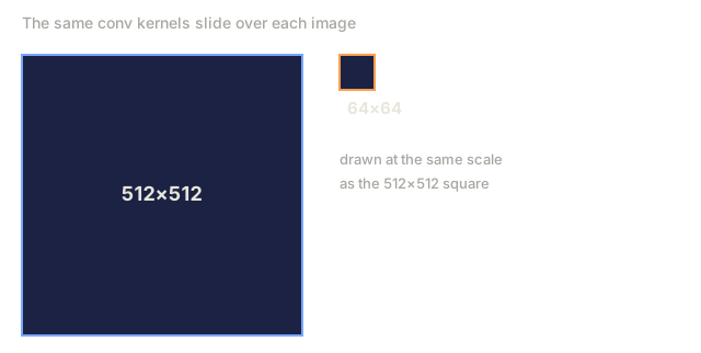
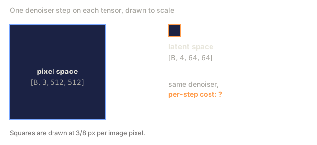
Latent diffusion is diffusion run on the compressed latent code of a VAE instead of on raw pixels. The reason to do it is cost. Pixel-space diffusion at 512² means the U-Net runs on tensors of shape [B, 3, 512, 512]. Each sampling step is ~100 GFLOPS for a 500M-param U-Net, so fifty steps is 5 TFLOPS per image. Train on a billion images and the compute bill is absurd.
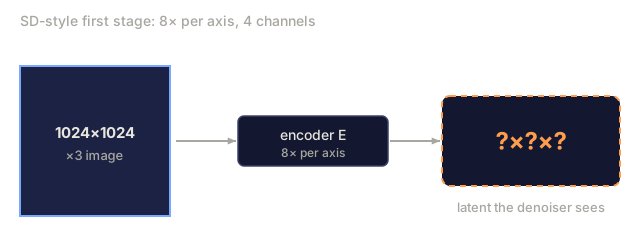
Most of those FLOPs go to pushing perceptually unimportant detail through the net, like the high-frequency texture a lossy VAE could compress away. Rombach's idea: train a VAE once (the first stage), freeze it, and run diffusion in the 4-channel 64×64 latent space (the second stage). Same U-Net, but 8× smaller along each axis (64×64 positions instead of 512×512, so 64× fewer spatial positions) and 4 latent channels instead of 3 pixel channels (~48× fewer values in total). Per-step compute falls by roughly the position-count factor, ~64×, for comparable quality.
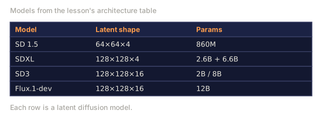
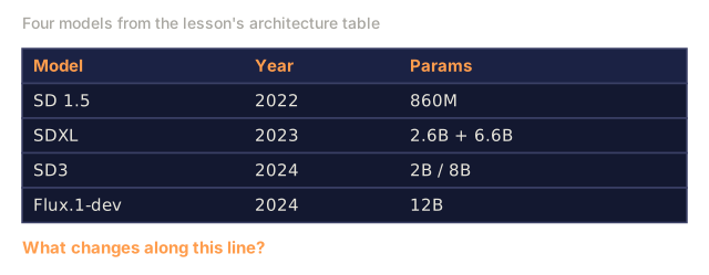
That is the Stable Diffusion recipe. SD 1.x / 2.x used an 860M U-Net over 64×64×4 latents, SDXL used a 2.6B U-Net over 128×128×4, and SD3 swapped the U-Net for a Diffusion Transformer (DiT) with flow matching. Flux.1-dev (Black Forest Labs, 2024) ships a 12B-param DiT-MMDiT. All of them run on the same two-stage substrate.
The Concept

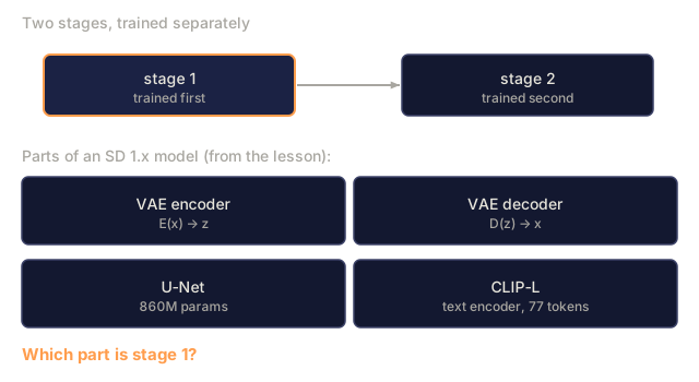
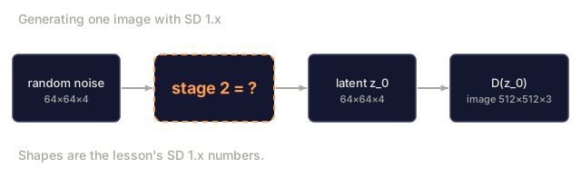
Latent diffusion splits generation into two stages, trained separately.
-
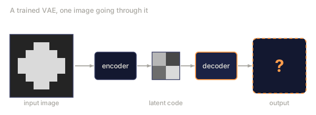
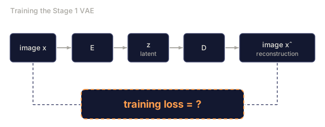
Stage 1: VAE. Encoder
E(x) → z, decoderD(z) → x. The target is 8× downsampling along each spatial axis, with a small channel count (4 for SD 1.x), so a 64×64×4 latent holds ~1/48 as many values as a 512×512×3 image. Loss = reconstruction (L1 + LPIPS perceptual) + KL. The KL weight is small sozisn't forced too close to Gaussian, since we don't need exact sampling fromz. An adversarial loss is often added so decoded images come out sharp. -
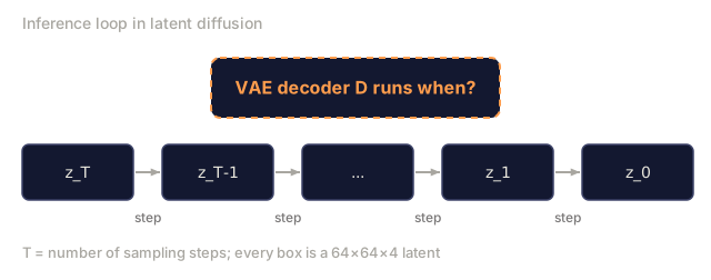
Stage 2: diffusion on
z. Treatz = E(x_real)as the data and train a U-Net (or DiT) to denoisez_t. At inference, samplez_0with diffusion, then decodex = D(z_0).
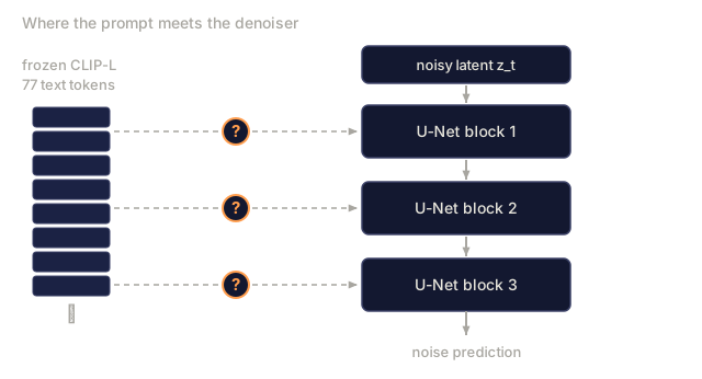
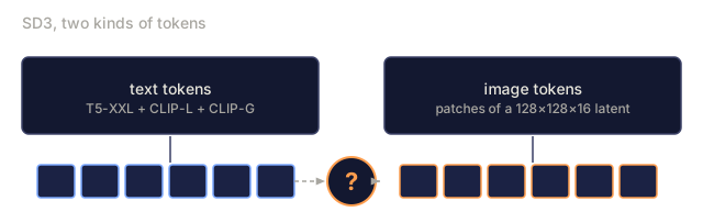
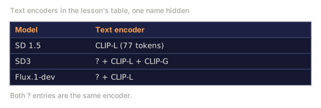
Text conditioning adds two components. A frozen text encoder produces the tokens (CLIP-L for SD 1.x, CLIP-L + OpenCLIP-G for SD 2/XL, T5-XXL for SD3 and Flux). Cross-attention injects them: each U-Net block takes [Q = image features, K = V = text tokens] and mixes them in. Text reaches the image through those tokens.
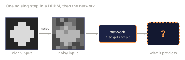
The loss function is identical to Lesson 06. Same DDPM / flow matching MSE on noise, with a different data domain underneath.
Architecture variants
| Model | Year | Backbone | Latent shape | Text encoder | Params |
|---|---|---|---|---|---|
| SD 1.5 | 2022 | U-Net | 64×64×4 | CLIP-L (77 tokens) | 860M |
| SD 2.1 | 2022 | U-Net | 64×64×4 | OpenCLIP-H | 865M |
| SDXL | 2023 | U-Net + refiner | 128×128×4 | CLIP-L + OpenCLIP-G | 2.6B + 6.6B |
| SDXL-Turbo | 2023 | Distilled | 128×128×4 | same | 1-4 step sampling |
| SD3 | 2024 | MMDiT (multimodal DiT) | 128×128×16 | T5-XXL + CLIP-L + CLIP-G | 2B / 8B |
| Flux.1-dev | 2024 | MMDiT | 128×128×16 | T5-XXL + CLIP-L | 12B |
| Flux.1-schnell | 2024 | MMDiT distilled | 128×128×16 | T5-XXL + CLIP-L | 12B, 1-4 step |
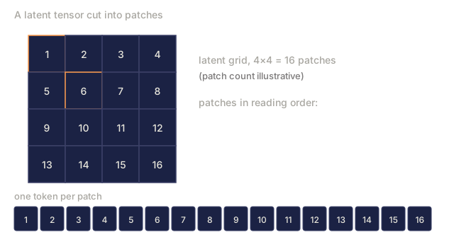
The trend across these models: U-Net gives way to DiT (a transformer over latent patches), the text encoder gets bigger (T5 beats CLIP for prompt adherence), and latent channels go up (4 → 16 gives more headroom for detail).
Build It
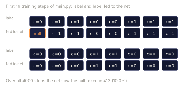
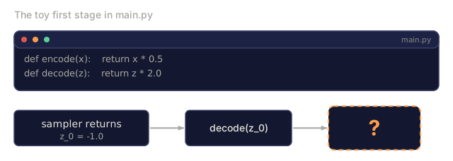
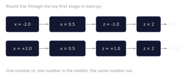
code/main.py stacks a toy 1-D first stage (a fixed rescale, encode(x) = 0.5x and decode(z) = 2z, standing in for a real conv-net VAE) under a small diffusion model and adds class conditioning with classifier-free guidance. The denoiser is a 2-hidden-layer tanh MLP with a hand-written backward pass, and the script carries its own linear beta schedule (T=40), so it needs no code from Lesson 06. It shows the key insight: the same diffusion loss works on raw 1-D values and on encoded values.
Step 1: encoder/decoder
def encode(x):    return x * 0.5          # toy "compression" to smaller scale
def decode(z):    return z * 2.0
A real VAE has trained weights. Here a linear map is enough to show that diffusion operates on z without caring about the original data space.
Step 2: diffusion in z-space
Same noise-prediction objective as Lesson 06, just with the script's own schedule and MLP in place of a U-Net. The data the net sees is z = E(x). After sampling z_0, decode with D(z_0).
Step 3: classifier-free guidance
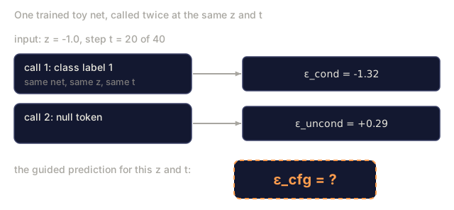
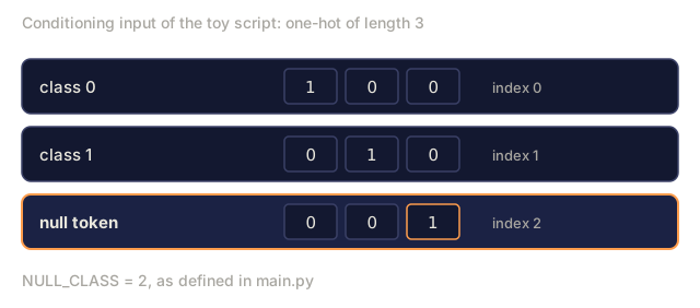
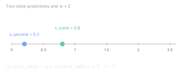
Classifier-free guidance blends a conditional and an unconditional prediction. During training, drop the class label 10% of the time (replace with a null token). At inference, compute both ε_cond and ε_uncond, then:
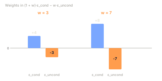
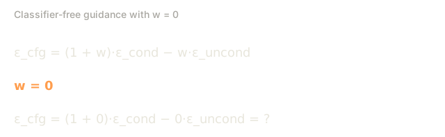
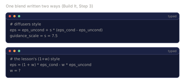
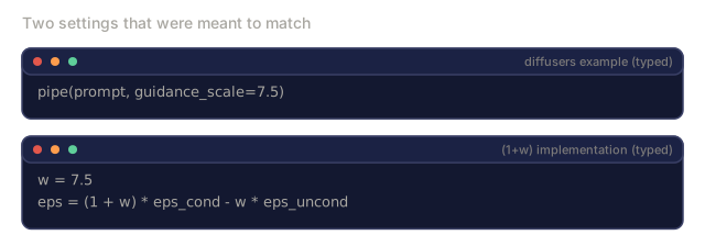
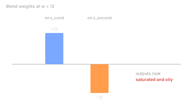
eps_cfg = (1 + w) * eps_cond - w * eps_uncondw = 0 is no guidance (the plain conditional prediction). This is the (1+w) form from Ho & Salimans, and it is what main.py computes. Many libraries write the same blend as eps_uncond + s * (eps_cond - eps_uncond) and call s the guidance scale. Expanding shows the two are identical when s = 1 + w: eps_uncond + (1 + w) * (eps_cond - eps_uncond) = (1 + w) * eps_cond - w * eps_uncond. So s = 1 is no guidance, and a diffusers guidance_scale of 7.5 is w = 6.5 here. The w values in this lesson (the sweep, the 3-7 range, the w > 10 warning) use the (1+w) convention. As a production rule of thumb, w around 3 is a common default and w of 7 or more starts to look saturated and over-sharp. The toy script does not measure either claim: it sweeps w in {0, 1, 3, 7} and prints the per-class mean over 200 samples at each setting.
Step 4: text conditioning (concept, not code)
Replace the class label with a frozen text encoder output. Feed the text embedding to the U-Net via cross-attention:
h = h + CrossAttention(Q=h, K=text_embed, V=text_embed)Swapping the class label for a text embedding and adding this attention step is what separates a class-conditional diffusion model from Stable Diffusion.
Pitfalls
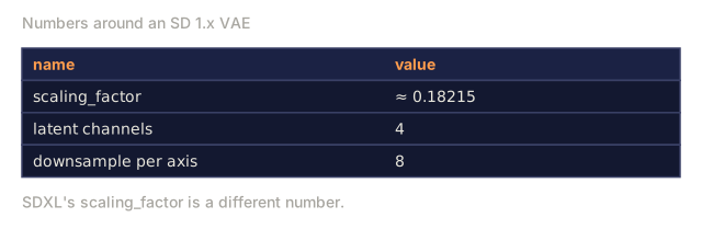
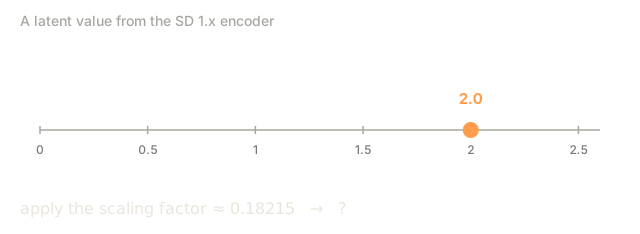
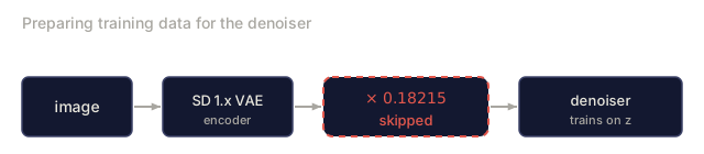
- VAE-scale mismatch. SD 1.x VAEs have a scaling constant (
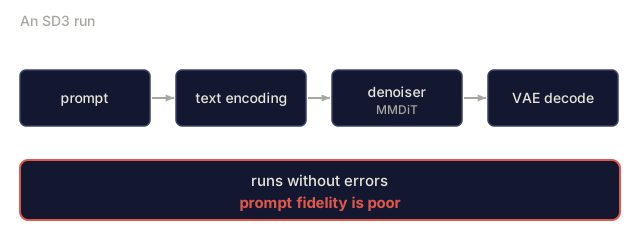
scaling_factor ≈ 0.18215) applied after encoding (you multiply the latents by it, which is the same as dividing by ~5.5). Forget it and the U-Net trains on latents with wildly wrong variance. Each VAE family has its own value (SDXL's differs from SD 1.x's), so read it from the checkpoint's config. - Text encoder silently wrong. SD3 needs T5-XXL with >=128 tokens, and the fallback to CLIP-only is lossy. Check
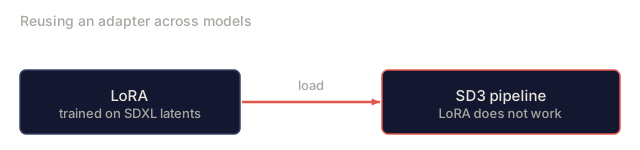
use_t5=True, or prompt fidelity craters. - Mixing latent spaces. SDXL, SD3, and Flux use different VAEs, so a LoRA trained on SDXL latents will not work on SD3. Hugging Face diffusers 0.30+ refuses to load mismatched checkpoints.
- CFG too high.
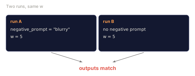
w > 10produces saturated, oily images and over-fits the prompt at the cost of diversity. The sweet spot isw = 3-7. - Negative prompts leaking. An empty negative prompt becomes the null token, while a filled one becomes
ε_uncond. These are different things, and some pipelines silently default to the null.
Use It
These are the production stacks in 2026, by target:
| Target | Recommended backbone |
|---|---|
| Narrow domain, paired data, training a model from scratch | SDXL fine-tune (LoRA / full), fastest to ship |
| Open-domain text-to-image, open weights | Flux.1-dev (12B, Apache / non-commercial) or SD3.5-Large |
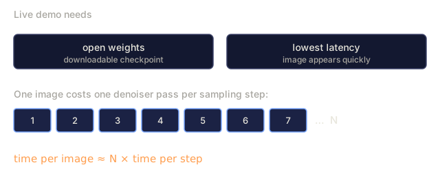
| Fastest inference, open weights | Flux.1-schnell (1-4 step, Apache) or SDXL-Lightning |
| Best prompt adherence, hosted | GPT-Image / DALL-E 3 (still), Midjourney v7, Imagen 4 |
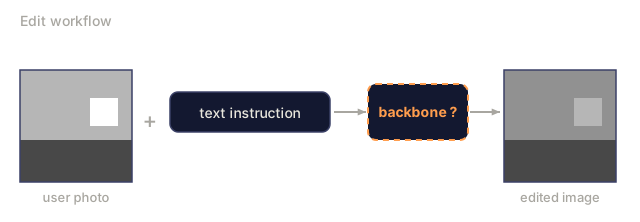
| Edit workflows | Flux.1-Kontext (Dec 2024), natively accepts image + text |
| Research, baseline | SD 1.5, ancient but well-studied |
Ship It
Save outputs/skill-sd-prompter.md. The skill takes a text prompt and a target style, and outputs a model + checkpoint, CFG scale, sampler, negative prompt, resolution, an optional ControlNet/IP-Adapter combo, and a per-step QA checklist.
I'd run the guidance sweep in main.py before reading anything else. The sample function evaluates the net twice per step, once with the class and once with the null class, then blends the two with w. Watching the per-class means as w goes from 0 to 7 is the quickest way I know to get a feel for what the scale does, and the whole script finishes in seconds in pure Python.
My bet is that the toy encoder hides what a real first stage adds. In the script, encode multiplies by 0.5 and decode multiplies by 2.0, so the round trip loses nothing. A learned VAE compresses, and the scaling-factor and mismatched-latent pitfalls above come from that stage, which the toy version skips. Exercise 2 is where I'd go next, since it swaps in a learned encoder with a reconstruction loss.
For the ship-it skill, I'd write the QA checklist straight from the pitfalls list: CFG range, how the negative prompt is handled, and whether the VAE matches the checkpoint.
Exercises
- Easy. Run
code/main.pywith the guidance sweepw ∈ {0, 1, 3, 7}(the script's own list). Compare the printed per-class means against the real data means of -2 and +2. At whatwdoes a class mean first move past its real mean? Then add15to the list and see whether the trend continues. - Medium. Swap the toy linear encoder for a tanh-MLP encoder/decoder pair with a reconstruction loss. Retrain diffusion on the new latents. Does sample quality change?
- Hard. Set up a real Stable Diffusion inference with diffusers: load
sdxl-base, run 30 Euler steps with CFG=7, time it. Now switch tosdxl-turbowith 4 steps and CFG=0. Same subject, different quality. Describe what changed and why.
Key Terms
| Term | What people say | What it actually means |
|---|---|---|
| First stage | "The VAE" | Trained encoder/decoder pair; compresses 512² to 64². |
| Second stage | "The U-Net" | Diffusion model over the latent space. |
| CFG | "Guidance scale" | (1+w)·ε_cond - w·ε_uncond; tunes conditioning strength. |
| Null token | "Empty prompt embed" | Unconditional embed used for ε_uncond. |
| Cross-attention | "How text gets in" | Each U-Net block attends to text tokens as K and V. |
| DiT | "Diffusion Transformer" | Replace U-Net with a transformer over latent patches; scales better. |
| MMDiT | "Multi-modal DiT" | SD3's architecture: text and image streams with joint attention. |
| VAE scaling factor | "Magic number" | Multiply latents by ~0.18215 after encoding (divide by ~5.5) so diffusion operates in roughly unit-variance space. |
Production note: running Flux-12B on an 8GB consumer GPU
The reference Flux integration is the canonical "I have a consumer GPU, can I ship this?" recipe. It applies the same three-knob recipe the production inference literature lists to a diffusion DiT:
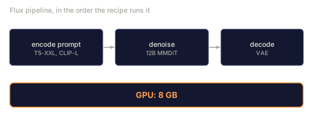
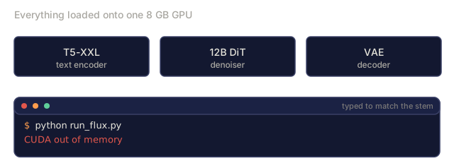
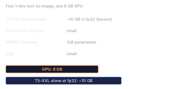
- Staggered loading. Flux has four networks that do not need to sit in VRAM at the same time: the T5-XXL text encoder (~10 GB in fp32), CLIP-L (small), the 12B MMDiT, and the VAE. Encode the prompt first, delete the encoders, load the DiT, denoise, delete the DiT, load the VAE, decode. A consumer 8GB GPU fits one stage at a time.
- 4-bit quantization via bitsandbytes. Use
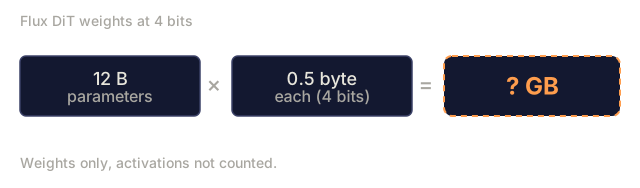
BitsAndBytesConfig(load_in_4bit=True, bnb_4bit_compute_dtype=torch.bfloat16)on both the T5 encoder and the DiT. It cuts memory 8×, and the quality drop is imperceptible for text-to-image per Aritra's benchmarks (linked in the notebook). - CPU offload.
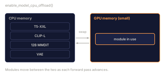
pipe.enable_model_cpu_offload()swaps modules between CPU and GPU as each forward pass advances. It adds 10-20% latency but lets the pipeline run at all.
The memory accounting: 10 GB T5 / 8 = 1.25 GB quantized, 12 B params × 0.5 bytes = ~6 GB for the quantized DiT, plus activations. In stas00's terms this is the extreme end of TP=1 inference, with no model parallelism and maximum quantization. For production you'd run TP=2 or TP=4 on H100s. For a single dev laptop, this is the recipe.
Further Reading
- Rombach et al. (2022). High-Resolution Image Synthesis with Latent Diffusion Models: Stable Diffusion.
- Podell et al. (2023). SDXL: Improving Latent Diffusion Models for High-Resolution Image Synthesis: SDXL.
- Peebles & Xie (2023). Scalable Diffusion Models with Transformers (DiT): DiT.
- Esser et al. (2024). Scaling Rectified Flow Transformers for High-Resolution Image Synthesis: SD3, MMDiT.
- Ho & Salimans (2022). Classifier-Free Diffusion Guidance: CFG.
- Labs (2024). Flux.1 — Black Forest Labs announcement: Flux.1 family.
- Hugging Face Diffusers docs: reference implementation for every checkpoint above.
Code
- main.py (python, 185 lines)