Diffusion Models — DDPM from Scratch
Diffusion destroys data with noise over many small steps (the DDPM paper uses about a thousand; the toy in this lesson uses 40), trains one neural net to predict that noise, and reverses the process at inference. Ho, Jain, Abbeel (2020) gave the field that recipe, and it stuck. Today most mainstream image, video, 3D, and music models run on this loop, sometimes with flow matching or consistency tricks on top.
Learning Objectives
- Write the closed-form forward step `q(x_t | x_0)` and use it to produce a noisy `x_t` from `x_0` in one line.
- Explain why the DDPM training loss regresses on the noise that was added, and why that gives one stable loss with no minimax.
- Implement a 1-D DDPM in pure Python: the beta schedule, a hand-written backward pass, and the reverse sampling loop.
- Choose between ε- and v-prediction, linear and cosine schedules, and DDIM-style fast samplers for a real diffusion setup.
The Problem
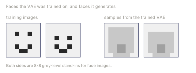
You want a sampler for p_data(x). GANs play a minimax game that often diverges. VAEs produce blurry samples from a Gaussian decoder. What you want is a training objective with three properties: (a) a single stable loss, with no saddle point and no minimax, (b) a lower bound on log p(x), so you have likelihoods, and (c) samples that match SOTA quality.
Sohl-Dickstein et al. (2015) had a theoretical answer: define a Markov chain q(x_t | x_{t-1}) that gradually adds Gaussian noise, and train a reverse chain p_θ(x_{t-1} | x_t) to denoise. Ho, Jain, Abbeel (2020) simplified the loss to one line, predict the noise, and cleaned up the math. In 2020 this was a curiosity. In 2021 it produced state-of-the-art samples. In 2022 it became Stable Diffusion. In 2026 it is the substrate.
The Concept
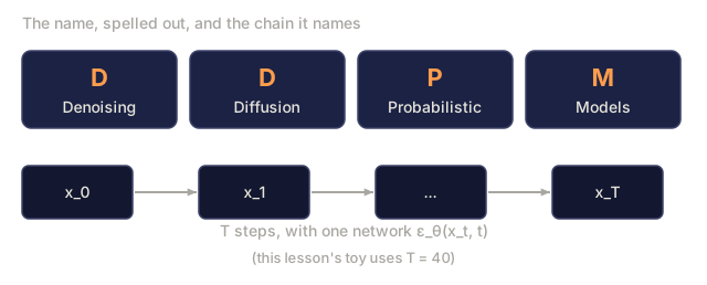
A denoising diffusion probabilistic model (DDPM) is a generative model built from two chains: a fixed forward process that turns data into Gaussian noise in small steps, and a learned reverse process that removes the noise one step at a time. One network, trained to predict the noise that was added, drives the reverse chain.

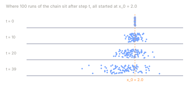
Forward process q. Add Gaussian noise in T small steps. The cumulative step also has a closed form because it is Gaussian, which is what makes the math tractable:
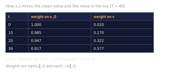
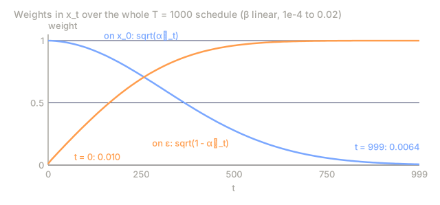
q(x_t | x_0) = N( sqrt(α̅_t) · x_0, (1 - α̅_t) · I )
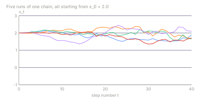
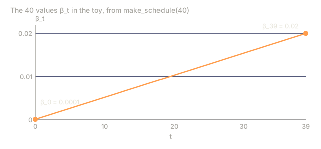
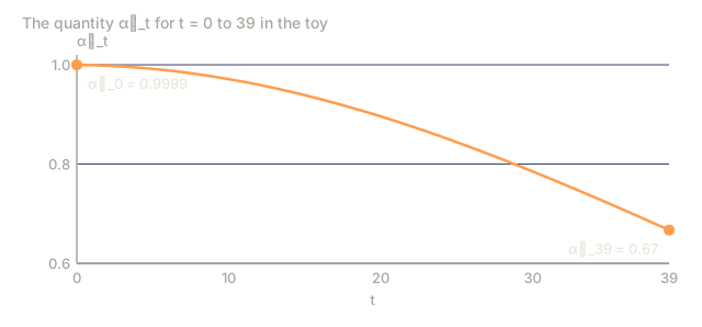
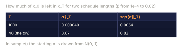
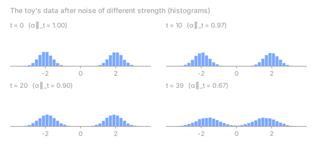
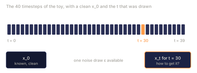
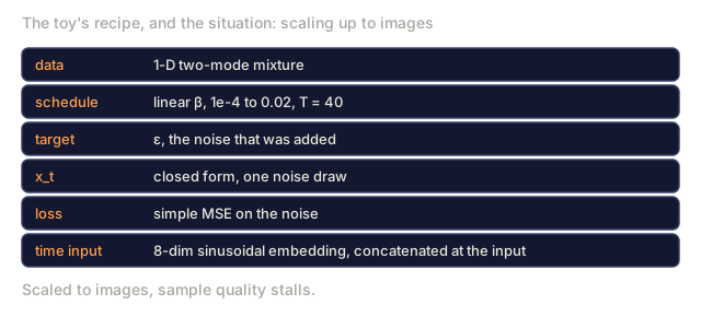
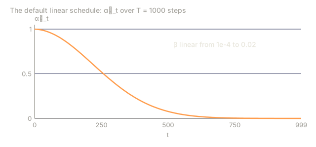
where α̅_t = ∏_{s=1..t} (1 - β_s) for a schedule of β_t. Pick β_t from 1e-4 to 0.02 linearly over T=1000 steps and x_T is approximately N(0, I). The toy in Build It is much shorter: it uses T=40 with the same β range, so α̅_T ≈ 0.67 and x_T still keeps about sqrt(0.67) ≈ 0.82 of the original signal. Its sample() starts from N(0, 1) anyway, a mismatch that a 1-D problem tolerates but real images would not.
Reverse process p_θ. Learn a neural net ε_θ(x_t, t) that predicts the noise that was added. Given x_t, denoise by:
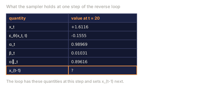
x_{t-1} = (1 / sqrt(α_t)) · ( x_t - (β_t / sqrt(1 - α̅_t)) · ε_θ(x_t, t) ) + σ_t · z
where σ_t is either sqrt(β_t) or a learned variance. The expression is ugly but it is just algebra, solving for x_{t-1} given the posterior q(x_{t-1} | x_t, x_0) and substituting x_0 with its noise-predicted estimate.
Training loss.
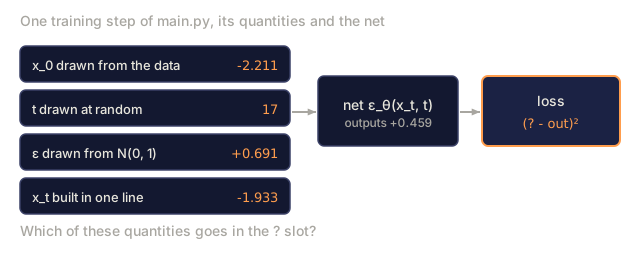
L_simple = E_{x_0, t, ε} [ || ε - ε_θ( sqrt(α̅_t) · x_0 + sqrt(1 - α̅_t) · ε, t ) ||² ]
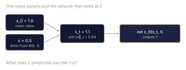
Sample x_0 from data, pick a random t, sample ε ~ N(0, I), compute the noisy x_t in one shot via the closed form, and regress on the noise. One loss, no minimax, no KL, no reparameterization tricks.
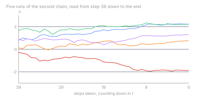
Sampling. Start x_T ~ N(0, I) and iterate the reverse step from t = T to 1. The final x is the sample.
Why it works
Three intuitions:
-
Denoising is easy; generating is hard. At
t=Tthe data is pure noise, so the net has a trivial problem to solve. Att=0it only has to clean up a few pixels. At intermediatetthe problem is hard, but the same weights get gradients from all noise levels. -
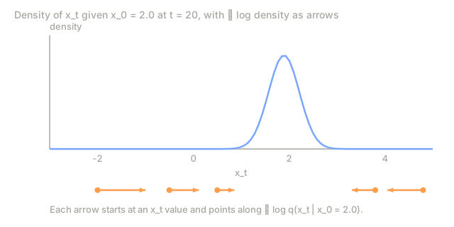
Score matching in disguise. Vincent (2011) proved that predicting the noise is equivalent to estimating
∇_x log q(x_t | x_0), the score. The reverse SDE uses this score to walk up the density gradient, a guided random walk toward high-probability regions. -
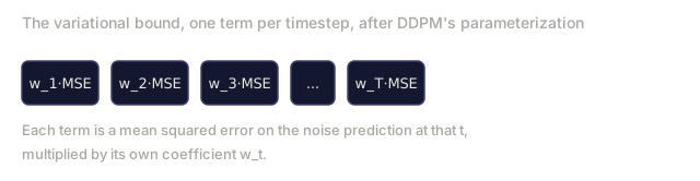
The ELBO reduces to simple MSE. The full variational lower bound has a KL term per timestep. With DDPM's parameterization those KL terms simplify to MSE on noise prediction with specific coefficients. Ho dropped the coefficients (calling it the "simple" loss) and quality improved.
Build It
main.py is a 1-D DDPM. The data is a two-mode mixture, and the "net" is a tiny MLP that takes (x_t, t) and outputs the predicted noise. Training is the one-line loss, and sampling iterates the reverse chain. The snippets below are illustrative; they follow main.py closely but compress it.
Step 1: the forward schedule (closed form)
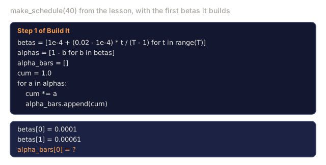
In main.py this lives in make_schedule(T), which returns (betas, alphas, alpha_bars).
betas = [1e-4 + (0.02 - 1e-4) * t / (T - 1) for t in range(T)]
alphas = [1 - b for b in betas]
alpha_bars = []
cum = 1.0
for a in alphas:
    cum *= a
    alpha_bars.append(cum)
Step 2: sample x_t in one shot
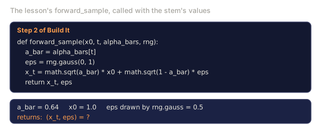
def forward_sample(x0, t, alpha_bars, rng):
    a_bar = alpha_bars[t]
    eps = rng.gauss(0, 1)
    x_t = math.sqrt(a_bar) * x0 + math.sqrt(1 - a_bar) * eps
    return x_t, eps
Step 3: one training step
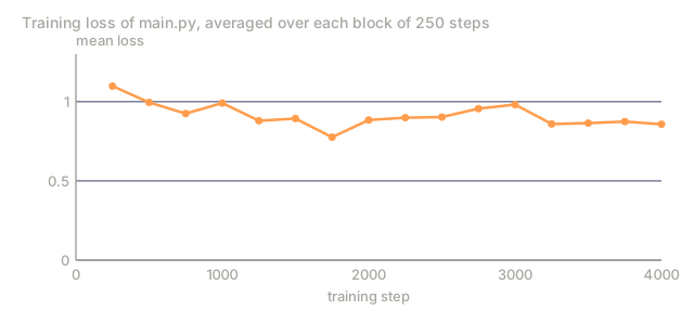
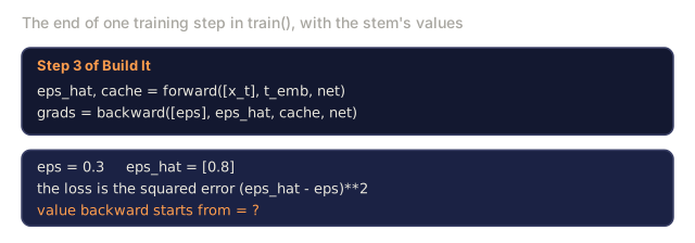
train() runs this inline for each update: draw a fresh x0 and a random t, build x_t with the closed form, embed t, run the forward pass, backprop by hand, and apply plain SGD. The loss (eps_hat - eps)**2 is only computed for printing, every 500 steps. The gradient backward uses is 2 * (eps_hat - eps) directly.
x0 = sample_data(rng)
t = rng.randrange(T)
x_t, eps = forward_sample(x0, t, alpha_bars, rng)   # Step 2, inlined in main.py
t_emb = sin_embed(t, T, t_dim)
eps_hat, cache = forward([x_t], t_emb, net)
grads = backward([eps], eps_hat, cache, net)
apply_update(net, grads, lr)
Step 4: reverse sampling
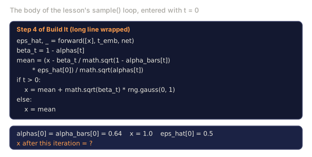
We need the full alphas list as well as alpha_bars, and the net needs the same time embedding it saw in training. The last step (t = 0) adds no fresh noise.
def sample(net, alphas, alpha_bars, T, t_dim, rng):
    x = rng.gauss(0, 1)
    for t in range(T - 1, -1, -1):
        t_emb = sin_embed(t, T, t_dim)
        eps_hat, _ = forward([x], t_emb, net)
        beta_t = 1 - alphas[t]
        mean = (x - beta_t / math.sqrt(1 - alpha_bars[t]) * eps_hat[0]) / math.sqrt(alphas[t])
        if t > 0:
            x = mean + math.sqrt(beta_t) * rng.gauss(0, 1)
        else:
            x = mean
    return x
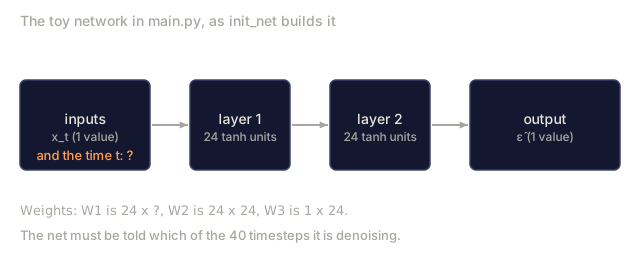
With 40 timesteps and a 24-unit MLP on this 1-D problem, main() trains for 4000 single-sample SGD updates (learning rate 0.01, one fresh x0 per step, no epochs). That is enough for 500 samples to land on both sides of zero, roughly 230 on the negative mode and 270 on the positive one.
Time conditioning
The net needs to know which timestep it is denoising. Two standard options:
- Sinusoidal embedding. Like Transformer positional encoding:
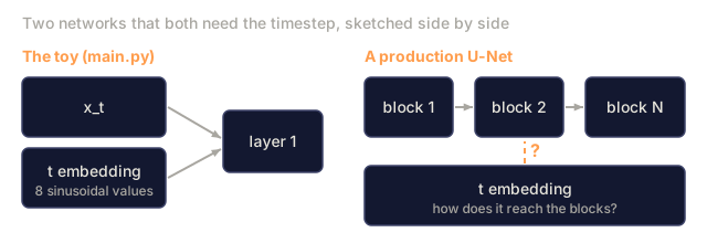
embed(t) = [sin(t/ω_0), cos(t/ω_0), sin(t/ω_1), ...]. The usual recipe passes it through a small MLP, then broadcasts the result into the net. - FiLM / group-norm conditioning. Project the embedding to per-channel scale and bias (FiLM) at each block.
The toy code skips the MLP: it concatenates the raw 8-dimensional sinusoidal vector (t_dim=8) onto x_t as the input to the first layer. Production U-Nets use FiLM.
Pitfalls
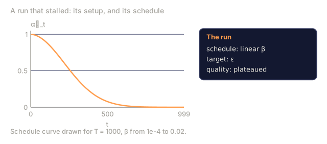
- Schedule matters a lot. Linear
βis the DDPM default, but the cosine schedule (Nichol & Dhariwal, 2021) gives better FID for the same compute. Switch schedules if quality plateaus. - Timestep embedding is fragile. Feeding raw
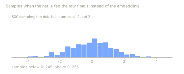
tas a float is a trap, which is why even the 1-D toy uses a sinusoidal embedding. Images need a proper embedding too, injected at every block. - V-prediction vs ε-prediction. For narrow regimes (very small or very large t),
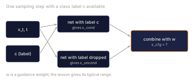
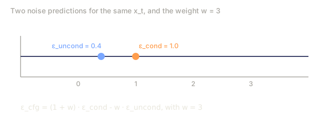
εhas poor signal-to-noise. V-prediction (v = α·ε - σ·x) is more stable, and Stable Diffusion 2.x (768-v) and Imagen Video use it. SDXL mostly predictsε, while SD3 and Flux predict a related velocity in a rectified-flow parameterization. - Classifier-free guidance. At inference, compute both conditional and unconditional
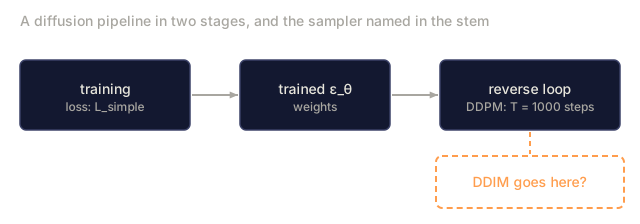
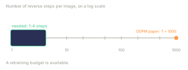
ε, thenε_cfg = (1 + w) · ε_cond - w · ε_uncondwithw ≈ 3-7. Covered in Lesson 08. - 1000 steps is a lot. Production uses DDIM (20-50 steps), DPM-Solver (10-20 steps), or distillation (1-4 steps). See Lesson 12.
Use It
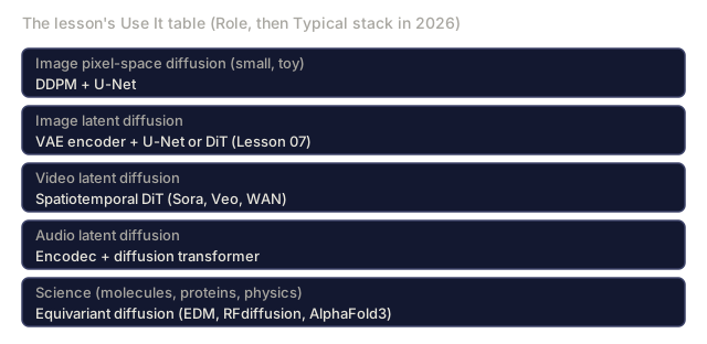
| Role | Typical stack in 2026 |
|---|---|
| Image pixel-space diffusion (small, toy) | DDPM + U-Net |
| Image latent diffusion | VAE encoder + U-Net or DiT (Lesson 07) |
| Video latent diffusion | Spatiotemporal DiT (Sora, Veo, WAN) |
| Audio latent diffusion | Encodec + diffusion transformer |
| Science (molecules, proteins, physics) | Equivariant diffusion (EDM, RFdiffusion, AlphaFold3) |
Diffusion is the generative backbone across all of these rows. Flow matching (Lesson 13) is the 2024-2026 competitor that usually wins on inference speed for the same quality.
Ship It
Save outputs/skill-diffusion-trainer.md. The skill takes a dataset and a compute budget and outputs a schedule (linear/cosine/sigmoid), prediction target (ε/v/x), number of steps, guidance scale, sampler family, and an eval protocol.
I'd run main.py before rereading the math. It trains on a 1-D two-mode mixture and prints a histogram plus a count of samples on each side of zero, so you can check by eye whether the reverse chain recovered both modes. The backward pass is hand-written, which means there is no framework between you and the loss.
My bet is that the closed-form forward step is the part worth rereading until it feels boring. In the training loop, x_t comes from x0, a_bar, and one draw of noise in a single line, with no loop over earlier steps. Once that clicks, the loss reads as plain regression on the noise you just added.
I'd also keep the toy in proportion. It uses the linear schedule and concatenates a sinusoidal embedding onto the input, which is a fine choice for a 1-D problem. On something bigger I'd try the cosine schedule and v-prediction from the Pitfalls list once quality plateaus, and use FiLM for time conditioning the way a real U-Net does.
Exercises
- Easy. Change
Tfrom 40 to 10 inmain()ofmain.py(it is a local variable there, passed tomake_schedule,train, andsample). How does sample quality (visual histogram of outputs) degrade? At what T does the two-mode structure collapse? - Medium. Switch from ε-prediction to v-prediction. Re-derive the reverse step. Compare final sample quality.
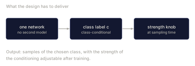
- Hard. Add classifier-free guidance. Condition on a class label
c ∈ {0, 1}, drop it 10% of the time during training, and at sampling time useε = (1+w)·ε_cond - w·ε_uncond. Measure the conditional-mode-hit rate atw = 0, 1, 3, 7.
Key Terms
| Term | What people say | What it actually means |
|---|---|---|
| Forward process | "Adding noise" | Fixed Markov chain q(x_t | x_{t-1}) that destroys the data. |
| Reverse process | "Denoising" | Learned chain p_θ(x_{t-1} | x_t) that reconstructs the data. |
| β schedule | "The noise ladder" | Per-step variance; linear, cosine, or sigmoid. |
| α̅ | "Alpha bar" | Cumulative product ∏(1 - β); gives closed-form x_t from x_0. |
| Simple loss | "MSE on noise" | ||ε - ε_θ(x_t, t)||²; all variational derivations collapse to this. |
| ε-prediction | "Predict noise" | Output is the noise added; standard DDPM. |
| V-prediction | "Predict velocity" | Output is α·ε - σ·x; better conditioning across t. |
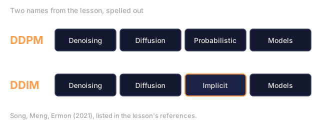
| DDPM | "The paper" | Ho et al. 2020; linear β, 1000 steps, U-Net. |
| DDIM | "Deterministic sampler" | Non-Markov sampler, 20-50 steps, same training objective. |
| Classifier-free guidance | "CFG" | Mix conditional and unconditional noise predictions to amplify conditioning. |
Production note: diffusion inference is a step-count problem
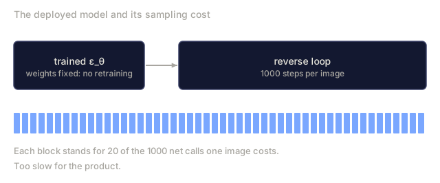
The DDPM paper runs T=1000 reverse steps. Production stacks rarely ship that. Real inference setups pick from three strategies, and each maps to a place the latency comes from:
- Faster sampler, same model. DDIM (20-50 steps), DPM-Solver++ (10-20), UniPC (8-16). It is a drop-in replacement for the reverse loop, and the trained
ε_θweights are untouched. Cuts latency 20-50×. - Distillation. Train a student to match the teacher in fewer steps: Progressive Distillation (2 → 1), Consistency Models (arbitrary → 1-4), LCM, SDXL-Turbo, SD3-Turbo. Cuts latency another 5-10× and requires retraining.
- Caching and compilation.
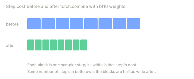
torch.compile(unet, mode="reduce-overhead"), TensorRT-LLM's diffusion backends,xformers/SDPA attention, bf16 weights. Cuts per-step latency ~2×. Stacks with (1) and (2).
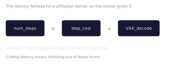
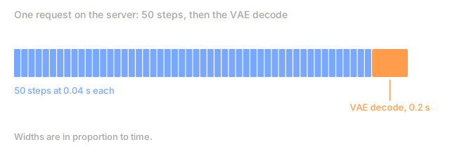
The budget conversation for a diffusion server mirrors the one for LLMs: latency is num_steps × step_cost + VAE_decode, and throughput is batch_size × (num_steps × step_cost)^-1. TTFT is small (one step). The TPOT equivalent is the full response time, because image generation is "all-at-once" from the user's perspective.
Further Reading
- Sohl-Dickstein et al. (2015). Deep Unsupervised Learning using Nonequilibrium Thermodynamics: the diffusion paper, ahead of its time.
- Ho, Jain, Abbeel (2020). Denoising Diffusion Probabilistic Models: DDPM.
- Song, Meng, Ermon (2021). Denoising Diffusion Implicit Models: DDIM, fewer steps.
- Nichol & Dhariwal (2021). Improved DDPM: cosine schedule, learned variance.
- Dhariwal & Nichol (2021). Diffusion Models Beat GANs on Image Synthesis: classifier guidance.
- Ho & Salimans (2022). Classifier-Free Diffusion Guidance: CFG.
- Karras et al. (2022). Elucidating the Design Space of Diffusion-Based Generative Models (EDM): unified notation, cleanest recipe.
Code
- main.py (python, 182 lines)