Image Generation — Diffusion Models
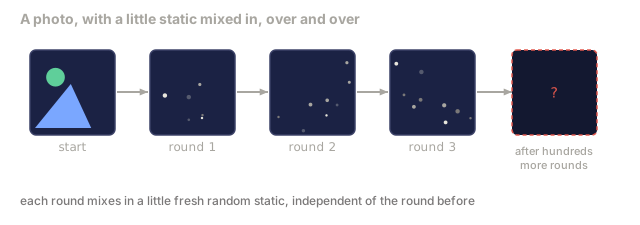
A diffusion model learns one trick: strip a little noise out of a noisy image. Run that trick backwards a thousand times starting from pure static, and an image appears.
Learning Objectives
- Derive the forward noising process `x_0 -> x_1 -> ... -> x_T` and explain why the closed-form `q(x_t | x_0)` holds for any t
- Implement a DDPM-style training objective that regresses the noise added at each step, and a sampler that walks back from pure noise to an image
- Build a time-conditioned U-Net (small enough to train on CPU) that predicts the noise for any timestep
- Explain the difference between DDPM and DDIM sampling, and when each is appropriate (Lesson 23 covers flow matching and rectified flow in depth)
The Problem
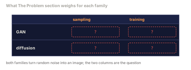
GANs generate in one shot: noise in, image out, a single forward pass. That makes them fast and famously hard to train. Diffusion models take the opposite trade: start from pure noise, denoise in small steps, and let the image emerge gradually. Slower, but far easier to train, and for the last five years that second property has won. Any small team can train a diffusion model and get reasonable samples — GAN training is still a craft you learn over years of failed runs.
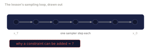
The bigger payoff is what diffusion's step-by-step structure unlocks: text conditioning, inpainting, image editing, super-resolution, controllable style. Every step in the sampling loop is a place to inject a new constraint, and that single hook is why Stable Diffusion, Imagen, DALL-E 3, Midjourney, and nearly every controllable image model you'll touch are built on diffusion.
This lesson builds the minimal version: forward noising, backward denoising, one training loop. The next lesson (Stable Diffusion) wires that core into a production system with a VAE, a text encoder, and classifier-free guidance.
The Concept
The forward process
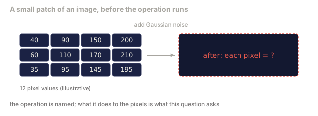
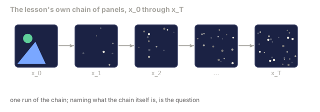
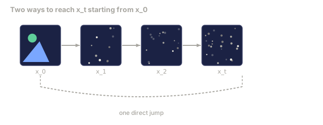
Take an image x_0. Add a tiny amount of Gaussian noise to get x_1. Add a tiny amount more to get x_2. Keep going for T steps until x_T is nearly indistinguishable from pure Gaussian noise.
q(x_t | x_{t-1}) = N(x_t; sqrt(1 - beta_t) * x_{t-1}, beta_t * I)
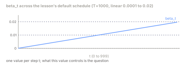
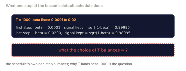
beta_t is a small variance schedule, typically linear from 0.0001 to 0.02 over T=1000 steps. Each step slightly shrinks the signal and injects fresh noise.
The closed-form jump
Adding noise one step at a time is a Markov chain (each step depends only on the state right before it, not the full history), but the math folds: you can sample x_t directly from x_0 in one step.
Define alpha_t = 1 - beta_t
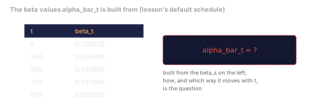
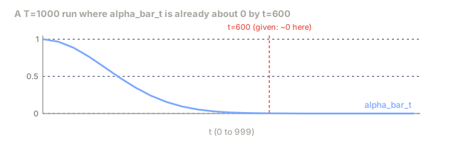
Define alpha_bar_t = prod_{s=1..t} alpha_s

Then:
  q(x_t | x_0) = N(x_t; sqrt(alpha_bar_t) * x_0,  (1 - alpha_bar_t) * I)

Equivalently:
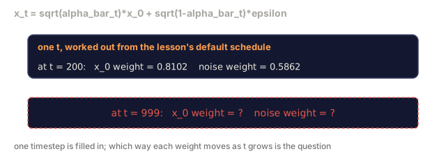
  x_t = sqrt(alpha_bar_t) * x_0 + sqrt(1 - alpha_bar_t) * epsilon
  where epsilon ~ N(0, I)
This single equation is the whole reason diffusion is practical: during training you pick a random t, sample x_t directly from x_0, and train in one step. No simulation of the full Markov chain required.
The reverse process
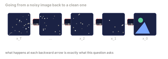
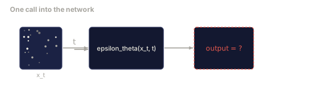
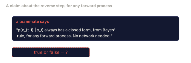
The forward process is fixed. The reverse process p(x_{t-1} | x_t) is what the neural network learns. Diffusion models do not predict x_{t-1} directly; they predict the noise epsilon added at step t, and the math derives x_{t-1} from it.

The training loss
For every training step:
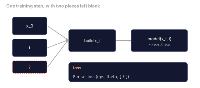
- Sample a real image
x_0. - Sample a timestep
tuniformly from [1, T]. - Sample noise
epsilon ~ N(0, I). - Compute
x_t = sqrt(alpha_bar_t) * x_0 + sqrt(1 - alpha_bar_t) * epsilon. - Predict
epsilon_theta(x_t, t)with the network. - Minimise
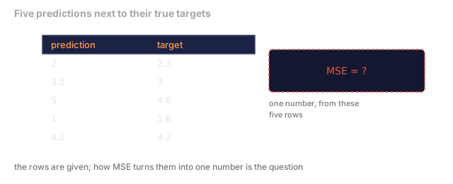
|| epsilon - epsilon_theta(x_t, t) ||^2.
That's it. The network learns to predict the noise at any timestep. The loss is plain MSE: no adversarial game, no collapse, no oscillation.
The sampler (DDPM)
To generate: start from x_T ~ N(0, I) and walk backwards one step at a time.
for t = T, T-1, ..., 1:
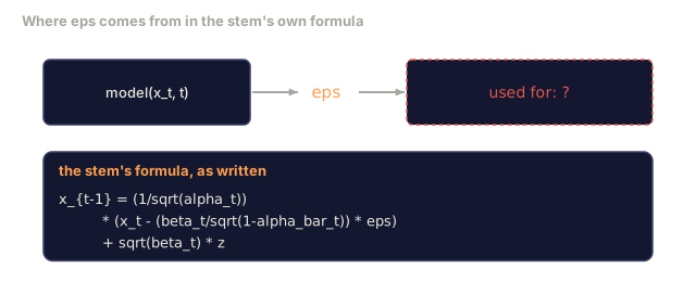
    eps = model(x_t, t)
    x_{t-1} = (1 / sqrt(alpha_t)) * (x_t - (beta_t / sqrt(1 - alpha_bar_t)) * eps) + sqrt(beta_t) * z
    where z ~ N(0, I) if t > 1, else 0
return x_0
In general, the reverse conditional has no closed form. For this specific Gaussian forward process, it does, and the ugly-looking coefficients above are exactly what Bayes' rule hands you.
Why 1000 steps
The forward noise schedule is chosen so each step adds just enough noise that the reverse step stays close to Gaussian. Too few steps and the reverse step drifts too far from Gaussian for the network to model well. Too many steps and sampling gets expensive for diminishing gain. T=1000 with a linear schedule is the DDPM default.
DDIM: 20x faster sampling
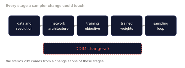
Training stays the same. Sampling changes. DDIM (Song et al., 2020) defines a deterministic reverse process that skips timesteps without retraining. Fifty steps with DDIM gets near-1000-step DDPM quality. Every production system uses DDIM or an even faster variant: DPM-Solver, Euler ancestral.
Time conditioning
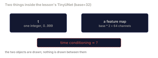
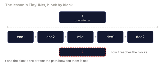
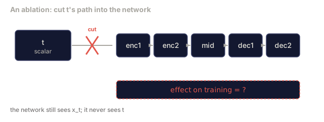
The network epsilon_theta(x_t, t) needs to know which timestep it's denoising. Modern diffusion models inject t via sinusoidal time embeddings: sine and cosine waves at a range of frequencies turn the scalar t into a vector, and that vector gets added to feature maps at every U-Net level. (You'll meet this exact trick again later in the curriculum as positional encoding in transformers.)
t_embedding = sinusoidal(t)
feature_map += MLP(t_embedding)
Skip time conditioning and the network has to guess the noise level from the image itself. That works, but it's far less sample-efficient.
Build It
Step 1: Noise schedule
import torch

def linear_beta_schedule(T=1000, beta_start=1e-4, beta_end=2e-2):
    return torch.linspace(beta_start, beta_end, T)


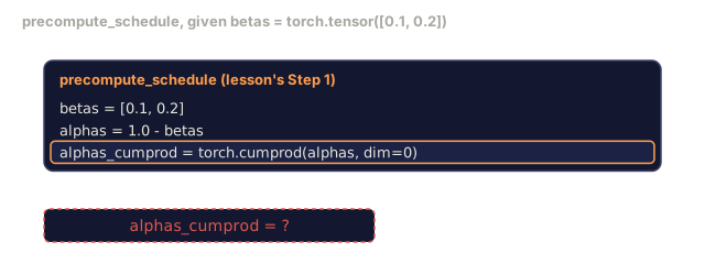
def precompute_schedule(betas):
    alphas = 1.0 - betas
    alphas_cumprod = torch.cumprod(alphas, dim=0)
    return {
        "betas": betas,
        "alphas": alphas,
        "alphas_cumprod": alphas_cumprod,
        "sqrt_alphas_cumprod": torch.sqrt(alphas_cumprod),
        "sqrt_one_minus_alphas_cumprod": torch.sqrt(1.0 - alphas_cumprod),
        "sqrt_recip_alphas": torch.sqrt(1.0 / alphas),
    }

schedule = precompute_schedule(linear_beta_schedule(T=1000))
Precompute once, gather by index during training and sampling.
Step 2: Forward diffusion (q_sample)
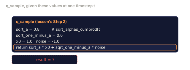
def q_sample(x0, t, noise, schedule):
    sqrt_a = schedule["sqrt_alphas_cumprod"][t].view(-1, 1, 1, 1)
    sqrt_one_minus_a = schedule["sqrt_one_minus_alphas_cumprod"][t].view(-1, 1, 1, 1)
    return sqrt_a * x0 + sqrt_one_minus_a * noise
One-line closed form. t is a batch of timesteps, one per image in the batch.
Step 3: A tiny time-conditioned U-Net
import torch.nn as nn
import torch.nn.functional as F
import math

def timestep_embedding(t, dim=64):
    half = dim // 2
    freqs = torch.exp(-math.log(10000) * torch.arange(half, device=t.device) / half)
    args = t[:, None].float() * freqs[None]
    emb = torch.cat([args.sin(), args.cos()], dim=-1)
    return emb


class TinyUNet(nn.Module):
    def __init__(self, img_channels=3, base=32, t_dim=64):
        super().__init__()
        self.t_mlp = nn.Sequential(
            nn.Linear(t_dim, base * 4),
            nn.SiLU(),
            nn.Linear(base * 4, base * 4),
        )
        self.t_dim = t_dim
        self.enc1 = nn.Conv2d(img_channels, base, 3, padding=1)
        self.enc2 = nn.Conv2d(base, base * 2, 4, stride=2, padding=1)
        self.mid = nn.Conv2d(base * 2, base * 2, 3, padding=1)
        self.dec1 = nn.ConvTranspose2d(base * 2, base, 4, stride=2, padding=1)
        self.dec2 = nn.Conv2d(base * 2, img_channels, 3, padding=1)
        self.time_proj = nn.Linear(base * 4, base * 2)

    def forward(self, x, t):
        t_emb = timestep_embedding(t, self.t_dim)
        t_emb = self.t_mlp(t_emb)
        t_proj = self.time_proj(t_emb)[:, :, None, None]

        h1 = F.silu(self.enc1(x))
        h2 = F.silu(self.enc2(h1)) + t_proj
        h3 = F.silu(self.mid(h2))
        d1 = F.silu(self.dec1(h3))
        d2 = torch.cat([d1, h1], dim=1)
        return self.dec2(d2)
Two-level U-Net with time conditioning injected at the bottleneck. Scale up the depth and width for real images.
Step 4: Training loop
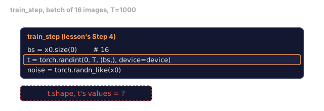
def train_step(model, x0, schedule, optimizer, device, T=1000):
    model.train()
    x0 = x0.to(device)
    bs = x0.size(0)
    t = torch.randint(0, T, (bs,), device=device)
    noise = torch.randn_like(x0)
    x_t = q_sample(x0, t, noise, schedule)
    pred = model(x_t, t)
    loss = F.mse_loss(pred, noise)
    optimizer.zero_grad()
    loss.backward()
    optimizer.step()
    return loss.item()
That's the entire training loop: no GAN game, no specialised loss, one MSE call.
Step 5: Sampler (DDPM)
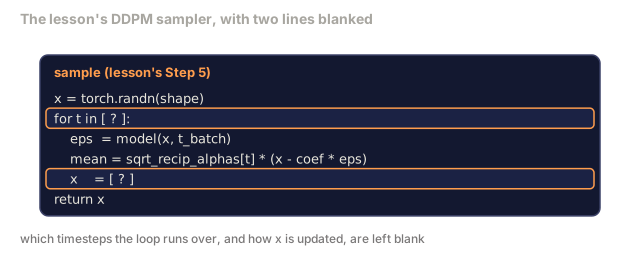
@torch.no_grad()
def sample(model, schedule, shape, T=1000, device="cpu"):
    model.eval()
    x = torch.randn(shape, device=device)
    betas = schedule["betas"].to(device)
    sqrt_one_minus_a = schedule["sqrt_one_minus_alphas_cumprod"].to(device)
    sqrt_recip_alphas = schedule["sqrt_recip_alphas"].to(device)

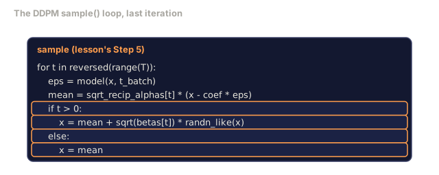
    for t in reversed(range(T)):
        t_batch = torch.full((shape[0],), t, dtype=torch.long, device=device)
        eps = model(x, t_batch)
        coef = betas[t] / sqrt_one_minus_a[t]
        mean = sqrt_recip_alphas[t] * (x - coef * eps)
        if t > 0:
            x = mean + torch.sqrt(betas[t]) * torch.randn_like(x)
        else:
            x = mean
    return x
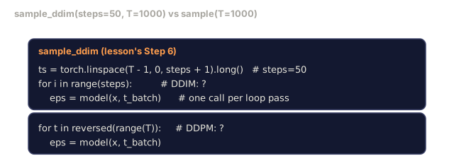
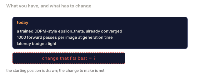
1000 forward passes to produce one batch of samples. In real code, you'd swap this for a DDIM 50-step sampler.
Step 6: DDIM sampler (deterministic, ~20x faster)
@torch.no_grad()
def sample_ddim(model, schedule, shape, steps=50, T=1000, device="cpu", eta=0.0):
    model.eval()
    x = torch.randn(shape, device=device)
    alphas_cumprod = schedule["alphas_cumprod"].to(device)

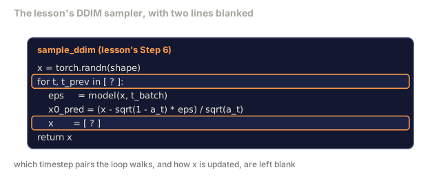
    ts = torch.linspace(T - 1, 0, steps + 1).long()
    for i in range(steps):
        t = ts[i]
        t_prev = ts[i + 1]
        t_batch = torch.full((shape[0],), t, dtype=torch.long, device=device)
        eps = model(x, t_batch)
        a_t = alphas_cumprod[t]
        a_prev = alphas_cumprod[t_prev] if t_prev >= 0 else torch.tensor(1.0, device=device)
        x0_pred = (x - torch.sqrt(1 - a_t) * eps) / torch.sqrt(a_t)
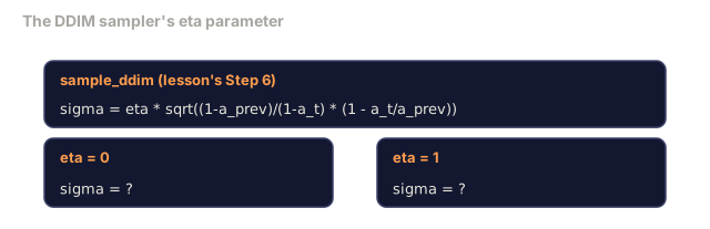
        sigma = eta * torch.sqrt((1 - a_prev) / (1 - a_t) * (1 - a_t / a_prev))
        dir_xt = torch.sqrt(1 - a_prev - sigma ** 2) * eps
        noise = sigma * torch.randn_like(x) if eta > 0 else 0
        x = torch.sqrt(a_prev) * x0_pred + dir_xt + noise
    return x
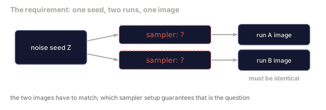
eta=0 is fully deterministic (same noise input always produces the same output). eta=1 recovers DDPM.
Use It
For production work, use diffusers:
from diffusers import DDPMScheduler, UNet2DModel

unet = UNet2DModel(sample_size=32, in_channels=3, out_channels=3, layers_per_block=2)
scheduler = DDPMScheduler(num_train_timesteps=1000)
The library ships ready-made schedulers (DDPM, DDIM, DPM-Solver, Euler, Heun), configurable U-Nets, pipelines for text-to-image and image-to-image, and LoRA fine-tuning helpers.
For research, k-diffusion (Katherine Crowson) has the most faithful reference implementations and the best sampling variants.
Ship It
This lesson produces:
outputs/prompt-diffusion-sampler-picker.md, a prompt that picks DDPM / DDIM / DPM-Solver / Euler based on quality target, latency budget, and conditioning type.outputs/skill-noise-schedule-designer.md, a skill that produces a linear, cosine, or sigmoid beta schedule given T and target corruption level, plus diagnostic plots of signal-to-noise ratio over time.
The detail that took me longest to actually believe: the network never predicts the image. It predicts the noise. The first time I saw the loss was just MSE against epsilon, my instinct was that something had to be missing, that the model needed some direct signal about what x_0 looked like. It doesn't, because the forward process is a plain linear equation, so predicting the noise and predicting the image are mathematically interchangeable. Epsilon-prediction just happens to give better-behaved gradients across the full noise range, especially near t = T, where predicting x_0 directly tends to blow up. If you ever train a diffusion model that looks fine at low t and falls apart near the end of the schedule, check the parameterization before you touch the architecture. That bug cost me a week the first time I hit it.
Exercises
- (Easy) Visualise the forward process: take one image and plot
x_tatt in [0, 100, 250, 500, 750, 1000]. Verify thatx_1000looks like pure Gaussian noise. - (Medium) Train the TinyUNet on the synthetic-circles dataset for 20 epochs and sample 16 circles. Compare DDPM (1000 steps) and DDIM (50 steps) sampling. Do they produce similar images from the same noise seed?
- (Hard) Implement a cosine noise schedule (Nichol & Dhariwal, 2021):
alpha_bar_t = cos^2((t/T + s) / (1 + s) * pi / 2). Train the same model with linear and cosine schedules and show that cosine gives better samples at low step counts.
Key Terms
| Term | What people say | What it actually means |
|---|---|---|
| Forward process | "Add noise over time" | Fixed Markov chain that corrupts an image into Gaussian noise over T steps |
| Reverse process | "Denoise step by step" | Learned distribution that walks back from noise to image |
| Epsilon prediction | "Predict the noise" | The training target: epsilon_theta(x_t, t) predicts the noise added at step t |
| Beta schedule | "Noise amounts" | Sequence of T small variances that define how much noise enters per step |
| alpha_bar_t | "Cumulative retain factor" | Product of (1 - beta_s) up to time t; bigger t means less signal left |
| DDPM sampler | "Ancestral, stochastic" | Samples each x_{t-1} from its conditional Gaussian; 1000 steps |
| DDIM sampler | "Deterministic, fast" | Rewrites sampling as a deterministic ODE; 20-100 steps with similar quality |
| Time conditioning | "Tell the model which t" | Sinusoidal embedding of t injected into the U-Net so it knows the noise level |
Further Reading
- Denoising Diffusion Probabilistic Models (Ho et al., 2020): the paper that made diffusion practical and beat GANs on FID
- Improved DDPM (Nichol & Dhariwal, 2021): cosine schedule and v-parameterisation
- DDIM (Song, Meng, Ermon, 2020): the deterministic sampler that made real-time inference possible
- Elucidating the Design Space of Diffusion (Karras et al., 2022): a unified view of every diffusion design choice; current best reference
Code
- main.py (python, 168 lines)