Stochastic Processes
Diffusion models, MCMC sampling, and RL exploration all run on the same trick: randomness with rules.
Learning Objectives
- Simulate 1D and 2D random walks and verify the sqrt(n) scaling of displacement
- Build a Markov chain simulator and compute its stationary distribution via eigendecomposition
- Implement Metropolis-Hastings MCMC and Langevin dynamics for sampling from target distributions
- Connect the forward diffusion process to Brownian motion and explain how the reverse process generates data
The Problem
A lot of AI systems run on randomness that evolves over time: not noise sitting still, but structured, sequential randomness where each step depends on the one before it.
Language models generate tokens one at a time, each conditioned on everything that came before. The model outputs a probability distribution, samples from it, and moves on. That's a stochastic process.
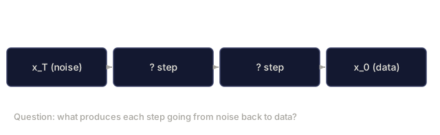
Diffusion models add noise to an image step by step until it's pure static, then reverse the process, denoising step by step until a new image emerges. The forward process is a Markov chain. The reverse process is a learned Markov chain running backward.
Reinforcement learning agents take actions in an environment, and each action leads to a new state with some probability. The agent follows a random policy through a random world: that's a Markov decision process.
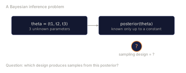
MCMC sampling, the backbone of Bayesian inference, constructs a Markov chain whose stationary distribution is the posterior you actually want to sample from.
Four ideas hold all of this up:
- Random walks, the simplest stochastic process.
- Markov chains, structured randomness with a transition matrix.
- Langevin dynamics, gradient descent with noise added in.
- Metropolis-Hastings, a way to sample from any distribution you can evaluate.
The Concept
Random Walks
A random walk is the simplest stochastic process there is: a position that moves by a random step at every tick, with no memory of anything except where it currently sits.
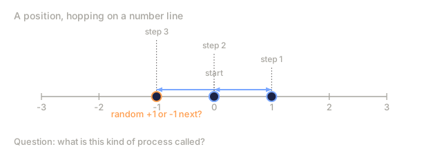
Here's the version everyone starts with. Begin at position 0. At each step, flip a fair coin: heads moves you right (+1), tails moves you left (-1).
After n steps, your position is the sum of n random +/-1 values. The expected position is 0, since the walk has no bias in either direction. But the expected distance from the origin grows as sqrt(n).
That's the counterintuitive part. The walk is fair, with no drift toward either side, and yet over time it wanders further and further from where it started. The standard deviation after n steps is exactly sqrt(n).
Step 0:  Position = 0
Step 1:  Position = +1 or -1
Step 2:  Position = +2, 0, or -2
...
Step 100: Expected distance from origin ~ 10 (sqrt(100))
Step 10000: Expected distance from origin ~ 100 (sqrt(10000))
In 2D, the walk moves up, down, left, or right with equal probability. The same sqrt(n) scaling applies to the distance from the origin, and the path it traces looks fractal.
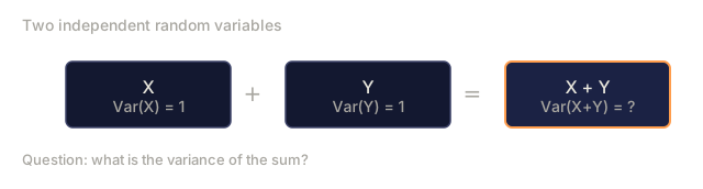
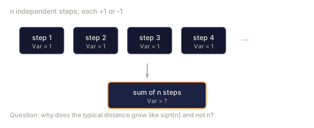
Why sqrt(n)? Each step is +1 or -1 with equal probability. After n steps, the position S_n = X_1 + X_2 + ... + X_n where each X_i is +/-1. Each step has variance 1, and the steps are independent, so Var(S_n) = n and the standard deviation is sqrt(n). By the central limit theorem, S_n / sqrt(n) converges to a standard normal distribution.
That sqrt(n) scaling shows up all over ML, not just here. SGD noise scales as 1/sqrt(batch_size). Embedding dimensions scale as sqrt(d). Whenever a square root shows up like this, it's usually the signature of independent random additions stacking on top of each other.
Connection to Brownian motion. Take a random walk with step size 1/sqrt(n) and n steps per unit time. As n goes to infinity, the walk converges to Brownian motion B(t): a continuous-time process where B(t) is normally distributed with mean 0 and variance t.
Brownian motion is the mathematical foundation of diffusion — it models the random jiggling of particles in a fluid, the fluctuations of stock prices, and, crucially, the noise process inside every diffusion model.
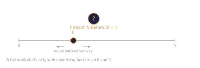
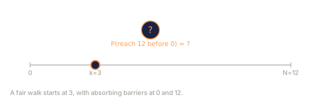
Gambler's ruin. Picture a random walker starting at position k, with absorbing barriers at 0 and N, so the walk stops the moment it hits either edge. What's the probability it reaches N before 0? For a fair walk, it's simply P(reach N) = k/N. That's a strikingly clean answer — it falls out of the theory of martingales: a fair random walk is a martingale, meaning its expected future value always equals its current value.
Markov Chains
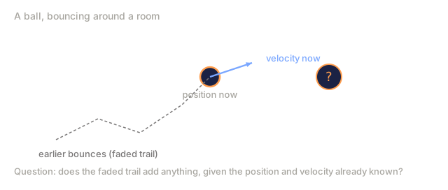
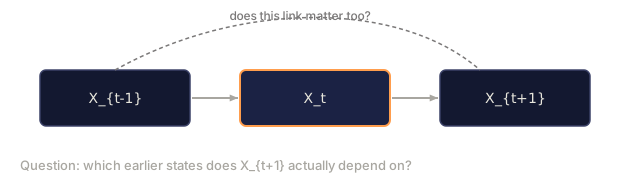
A Markov chain is a system that hops between states according to fixed probabilities, with one defining rule: the next state depends only on the current state, never on the history that got you there.
P(X_{t+1} = j | X_t = i, X_{t-1} = ...) = P(X_{t+1} = j | X_t = i)
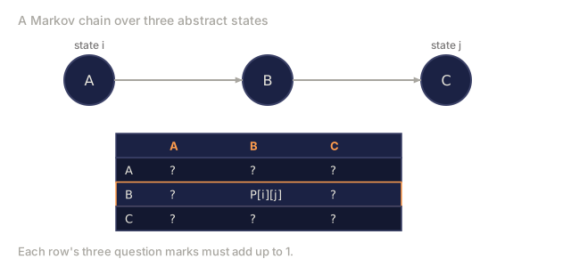
That's the Markov property, and it's what lets you describe the entire dynamics with a single transition matrix P:
P[i][j] = probability of going from state i to state j
Each row of P sums to 1, because you have to go somewhere.
Example, weather:
States: Sunny (0), Rainy (1), Cloudy (2)

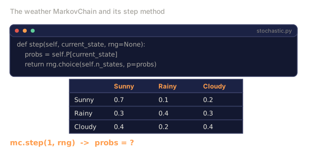
P = [[0.7, 0.1, 0.2],    (if sunny: 70% sunny, 10% rainy, 20% cloudy)
     [0.3, 0.4, 0.3],    (if rainy: 30% sunny, 40% rainy, 30% cloudy)
     [0.4, 0.2, 0.4]]    (if cloudy: 40% sunny, 20% rainy, 40% cloudy)
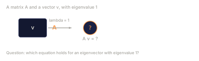
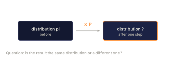
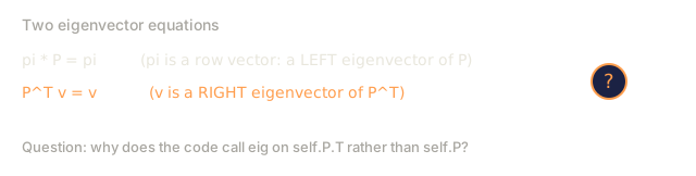
Start in any state and run this forward. After many transitions, the distribution of states converges to the stationary distribution pi, where pi * P = pi: the left eigenvector of P with eigenvalue 1.
For the weather chain, that stationary distribution might work out to [0.53, 0.18, 0.29]. Over the long run, it's sunny 53% of the time no matter where you started.

Computing the stationary distribution takes one of two approaches:
- Power method: multiply any initial distribution by P repeatedly. After enough iterations, it converges.
- Eigenvalue method: find the left eigenvector of P with eigenvalue 1, the same as the eigenvector of P^T with eigenvalue 1.
Both need the chain to satisfy a couple of convergence conditions first.
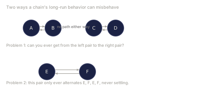
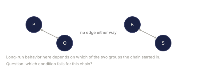
Convergence conditions. A Markov chain converges to a unique stationary distribution if it's:
- Irreducible: every state is reachable from every other state.
- Aperiodic: the chain doesn't cycle with a fixed period.
Most chains you'll run into in ML satisfy both.
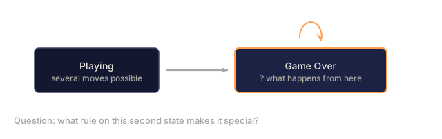
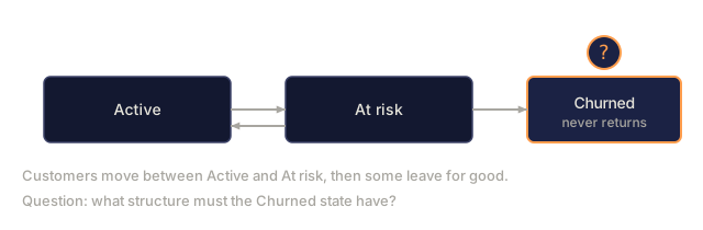
Absorbing states. A state is absorbing if once you enter it, you never leave: P[i][i] = 1. Absorbing Markov chains model processes with terminal states: a game that ends, a customer who churns, a token sequence that hits the end-of-text token.
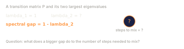
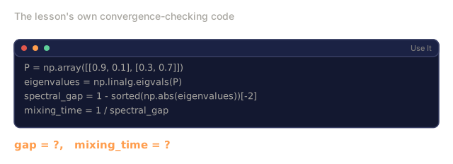
Mixing time asks how many steps it takes until the chain is "close" to its stationary distribution, formally the number of steps until the total variation distance from stationarity drops below some threshold. Fast mixing means few steps needed. The spectral gap of P (1 minus the second-largest eigenvalue) controls it directly: the larger the gap, the faster the chain mixes.
Connection to Language Models
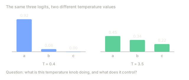
Token generation in a language model is, approximately, a Markov process: given the current context, the model outputs a distribution over the next token, and temperature controls how sharp that distribution is.
P(token_i) = exp(logit_i / temperature) / sum(exp(logit_j / temperature))
- Temperature = 1.0: the standard distribution.
- Temperature < 1.0: sharper, more deterministic.
- Temperature > 1.0: flatter, more random.
- Temperature -> 0: argmax, fully greedy.
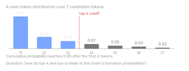
Top-k sampling truncates to the k highest-probability tokens. Top-p (nucleus) sampling truncates to the smallest set of tokens whose cumulative probability clears p. Both are just different ways of reshaping the Markov transition probabilities before you sample.
Brownian Motion
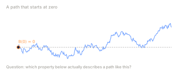
Brownian motion is the continuous-time limit of the random walk. Its position B(t) is defined by three properties:
- B(0) = 0.
- B(t) - B(s) is normally distributed with mean 0 and variance t - s, for t > s.
- Increments on non-overlapping intervals are independent.
It's continuous everywhere but differentiable nowhere: it jiggles at every scale you zoom into, which is also why its path has fractal dimension 2 in the plane.
In discrete simulation, you approximate it step by step:
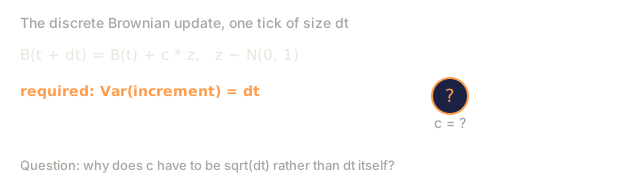
B(t + dt) = B(t) + sqrt(dt) * z, where z ~ N(0, 1)
That sqrt(dt) scaling isn't a rounding choice. It falls directly out of the central limit theorem applied to random walks.
Langevin Dynamics
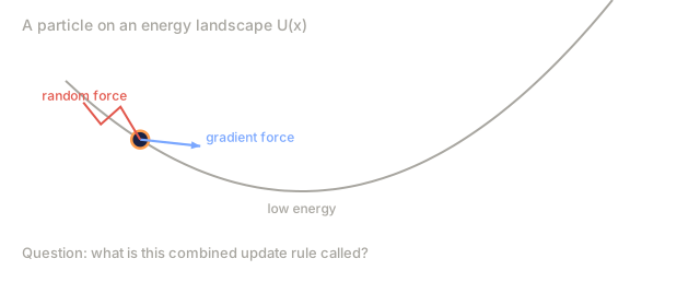
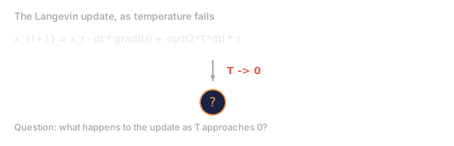
Where gradient descent finds a minimum of a function, Langevin dynamics finds an entire probability distribution: one proportional to exp(-U(x)/T), where U is an energy function and T is temperature.
x_{t+1} = x_t - dt * gradient(U(x_t)) + sqrt(2 * T * dt) * z_t
Two forces act on the particle at every step:
- Gradient force (-dt * gradient(U)): pushes toward low energy, exactly like gradient descent.
- Random force (sqrt(2Tdt) * z): pushes in a random direction, forcing exploration.
At temperature T = 0, this collapses to pure gradient descent. At high temperature, it's nearly a random walk. Somewhere in between, the particle explores the whole energy landscape while still spending more of its time in the low-energy regions.
Connection to diffusion models. The forward process of a diffusion model runs on the same idea:
x_t = sqrt(alpha_t) * x_{t-1} + sqrt(1 - alpha_t) * noise
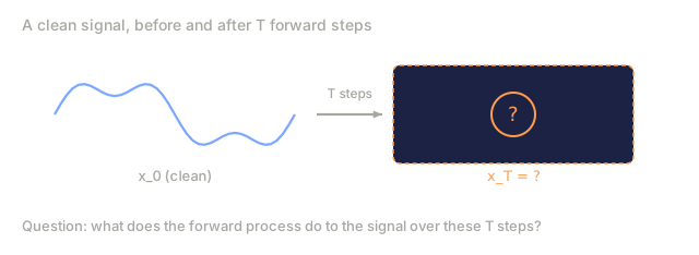
This is a Markov chain that gradually mixes the data with noise, until after enough steps x_T is pure Gaussian noise.
Running that backward, from noise to data, is also a Markov chain — just one whose transition probabilities are learned by a neural network instead of fixed by a formula. The network learns to predict the noise that was added at each step, then subtracts it out.

MCMC: Markov Chain Monte Carlo
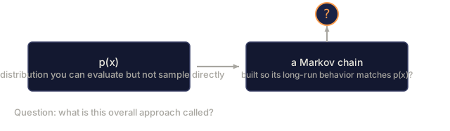
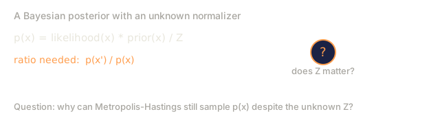
MCMC, Markov Chain Monte Carlo, builds a Markov chain whose stationary distribution is the exact distribution you're trying to sample from — that's the whole trick. You reach for it whenever you have a distribution p(x) you can evaluate, at least up to a constant, but can't sample from directly. Bayesian posteriors are the classic example: you know the likelihood times the prior, but the normalizing constant is intractable.
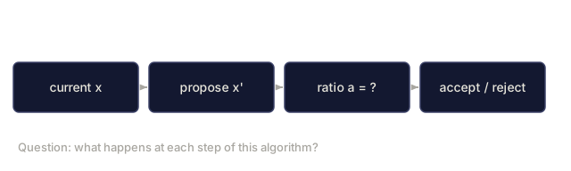
Metropolis-Hastings is the standard way to build that chain:
- Start at some position x.
- Propose a new position x' from a proposal distribution Q(x'|x).
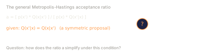
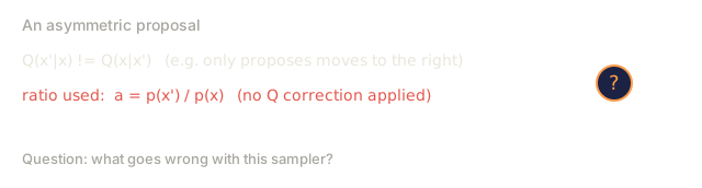
- Compute the acceptance ratio: a = p(x') * Q(x|x') / (p(x) * Q(x'|x)).
- Accept x' with probability min(1, a). Otherwise stay at x.
- Repeat.
If Q is symmetric (say Q(x'|x) = Q(x|x') = N(x, sigma^2)), the ratio simplifies to a = p(x') / p(x): you only need the ratio of probabilities, since the normalizing constant cancels out entirely.
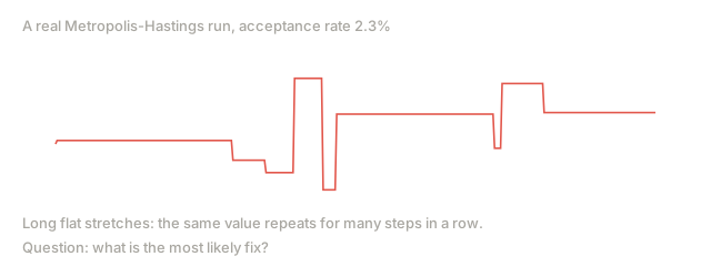
The chain is guaranteed to converge to p(x) under mild conditions, but convergence can be slow if the proposal is too small (it behaves like a random walk) or too large (too much gets rejected). Tuning the proposal well is most of what makes MCMC an art rather than a formula.
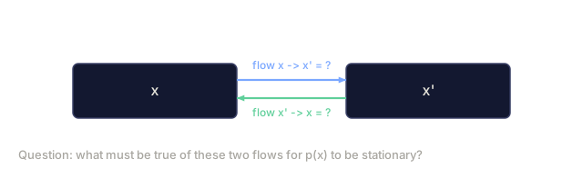
Why it works. The acceptance ratio enforces detailed balance: the probability of being at x and moving to x' equals the probability of being at x' and moving to x. Detailed balance is what guarantees p(x) is the chain's stationary distribution, so after enough steps, the samples you're collecting really do come from p(x).
Practical considerations:
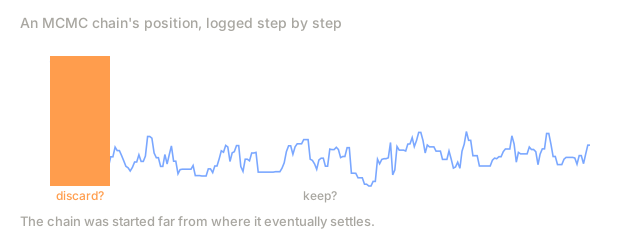
- Burn-in: discard the first N samples, since the chain needs time to reach the stationary distribution from wherever it started.
- Thinning: keep every k-th sample to cut down autocorrelation.
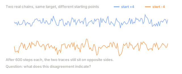
- Multiple chains: run several chains from different starting points. If they all converge to the same distribution, that's evidence you've actually converged.
- Acceptance rate: for Gaussian proposals in d dimensions, the optimal acceptance rate sits around 23% (Roberts & Rosenthal, 2001). Too high and the chain barely moves; too low and it rejects nearly everything.
Stochastic Processes in AI
| Process | AI Application |
|---|---|
| Random walk | Exploration in RL, Node2Vec embeddings |
| Markov chain | Text generation, MCMC sampling |
| Brownian motion | Diffusion models (forward process) |
| Langevin dynamics | Score-based generative models, SGLD |
| Markov decision process | Reinforcement learning |
| Metropolis-Hastings | Bayesian inference, posterior sampling |
Build It
Step 1: Random walk simulator
import numpy as np

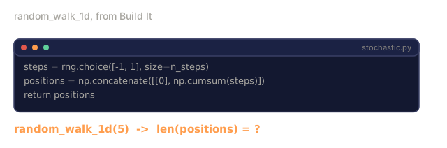
def random_walk_1d(n_steps, seed=None):
    rng = np.random.RandomState(seed)
    steps = rng.choice([-1, 1], size=n_steps)
    positions = np.concatenate([[0], np.cumsum(steps)])
    return positions


def random_walk_2d(n_steps, seed=None):
    rng = np.random.RandomState(seed)
    directions = rng.choice(4, size=n_steps)
    dx = np.zeros(n_steps)
    dy = np.zeros(n_steps)
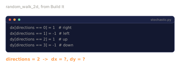
    dx[directions == 0] = 1   # right
    dx[directions == 1] = -1  # left
    dy[directions == 2] = 1   # up
    dy[directions == 3] = -1  # down
    x = np.concatenate([[0], np.cumsum(dx)])
    y = np.concatenate([[0], np.cumsum(dy)])
    return x, y
The 1D walk stores cumulative sums: each step is +1 or -1, and after n steps the position is just the running sum. Because the variance grows linearly with n, the standard deviation grows as sqrt(n).
Step 2: Markov chain
class MarkovChain:
    def __init__(self, transition_matrix, state_names=None):
        self.P = np.array(transition_matrix, dtype=float)
        self.n_states = len(self.P)
        self.state_names = state_names or [str(i) for i in range(self.n_states)]

    def step(self, current_state, rng=None):
        if rng is None:
            rng = np.random.RandomState()
        probs = self.P[current_state]
        return rng.choice(self.n_states, p=probs)

    def simulate(self, start_state, n_steps, seed=None):
        rng = np.random.RandomState(seed)
        states = [start_state]
        current = start_state
        for _ in range(n_steps):
            current = self.step(current, rng)
            states.append(current)
        return states

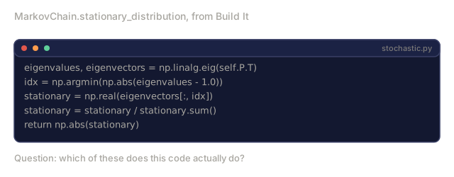
    def stationary_distribution(self):
        eigenvalues, eigenvectors = np.linalg.eig(self.P.T)
        idx = np.argmin(np.abs(eigenvalues - 1.0))
        stationary = np.real(eigenvectors[:, idx])
        stationary = stationary / stationary.sum()
        return np.abs(stationary)
The stationary distribution is the left eigenvector of P with eigenvalue 1. We get it by computing eigenvectors of P^T instead, since transposing turns left eigenvectors into right eigenvectors that NumPy can compute directly.
Step 3: Langevin dynamics
def langevin_dynamics(grad_U, x0, dt, temperature, n_steps, seed=None):
    rng = np.random.RandomState(seed)
    x = np.array(x0, dtype=float)
    trajectory = [x.copy()]
    for _ in range(n_steps):
        noise = rng.randn(*x.shape)
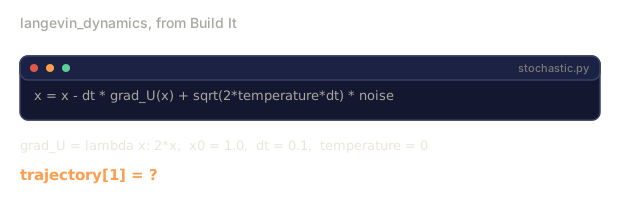
        x = x - dt * grad_U(x) + np.sqrt(2 * temperature * dt) * noise
        trajectory.append(x.copy())
    return np.array(trajectory)
The gradient pulls x toward low energy; the noise keeps it from getting stuck in one place. At equilibrium, the samples you collect follow a distribution proportional to exp(-U(x)/temperature).
Step 4: Metropolis-Hastings
def metropolis_hastings(target_log_prob, proposal_std, x0, n_samples, seed=None):
    rng = np.random.RandomState(seed)
    x = np.array(x0, dtype=float)
    samples = [x.copy()]
    accepted = 0
    for _ in range(n_samples - 1):
        x_proposed = x + rng.randn(*x.shape) * proposal_std
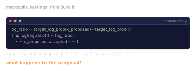
        log_ratio = target_log_prob(x_proposed) - target_log_prob(x)
        if np.log(rng.rand()) < log_ratio:
            x = x_proposed
            accepted += 1
        samples.append(x.copy())
    acceptance_rate = accepted / (n_samples - 1)
    return np.array(samples), acceptance_rate
The algorithm proposes a new point, checks whether it's more probable (or accepts anyway with probability proportional to the ratio), and repeats. Aim for an acceptance rate around 23 to 50 percent for good mixing.
Use It
In practice, you'll reach for established libraries instead of hand-rolling any of this. But the mechanics still matter, because debugging a slow or broken sampler means knowing what's actually happening underneath the library call.
import numpy as np

rng = np.random.RandomState(42)
walk = np.cumsum(rng.choice([-1, 1], size=10000))
print(f"Final position: {walk[-1]}")
print(f"Expected distance: {np.sqrt(10000):.1f}")
print(f"Actual distance: {abs(walk[-1])}")
numpy for transition matrices
import numpy as np

P = np.array([[0.7, 0.1, 0.2],
              [0.3, 0.4, 0.3],
              [0.4, 0.2, 0.4]])

distribution = np.array([1.0, 0.0, 0.0])
for _ in range(100):
    distribution = distribution @ P

print(f"Stationary distribution: {np.round(distribution, 4)}")
Multiply the initial distribution by P repeatedly, and after enough iterations it converges to the stationary distribution no matter where you started. That's the power method for finding the dominant left eigenvector, working in code exactly the way it works on paper.
Connections to real frameworks
- PyTorch diffusion: The
DDPMSchedulerin Hugging Facediffusersimplements the forward and reverse Markov chains. - NumPyro / PyMC: Use MCMC (the NUTS sampler, an improvement on Metropolis-Hastings) for Bayesian inference.
- Gymnasium (RL): The environment's step function defines a Markov decision process.
Verifying Markov chain convergence
import numpy as np

P = np.array([[0.9, 0.1], [0.3, 0.7]])

eigenvalues = np.linalg.eigvals(P)
spectral_gap = 1 - sorted(np.abs(eigenvalues))[-2]
print(f"Eigenvalues: {eigenvalues}")
print(f"Spectral gap: {spectral_gap:.4f}")
print(f"Approximate mixing time: {1/spectral_gap:.1f} steps")
The spectral gap tells you how fast the chain forgets its initial state: a gap of 0.2 means roughly 5 steps to mix, a gap of 0.01 means roughly 100. Check this before running a long simulation. A slowly mixing chain just burns compute for no benefit.
Ship It
This lesson produces:
outputs/prompt-stochastic-process-advisor.md, a prompt that helps identify which stochastic process framework applies to a given problem
Connections
| Concept | Where it shows up |
|---|---|
| Random walk | Node2Vec graph embeddings, exploration in RL |
| Markov chain | Token generation in LLMs, MCMC sampling |
| Brownian motion | Forward diffusion process in DDPM, SDE-based models |
| Langevin dynamics | Score-based generative models, stochastic gradient Langevin dynamics (SGLD) |
| Stationary distribution | MCMC convergence target, PageRank |
| Metropolis-Hastings | Bayesian posterior sampling, simulated annealing |
| Temperature | LLM sampling, Boltzmann exploration in RL, simulated annealing |
| Mixing time | Convergence speed of MCMC, spectral gap analysis |
| Absorbing state | End-of-sequence token, terminal states in RL |
| Detailed balance | Correctness guarantee for MCMC samplers |
Diffusion models deserve special attention here. DDPM (Ho et al., 2020) defines a forward Markov chain:
q(x_t | x_{t-1}) = N(x_t; sqrt(1-beta_t) * x_{t-1}, beta_t * I)
where beta_t is a noise schedule (alpha_t = 1 - beta_t, the same schedule as the alpha_t formula above), and after T steps x_T is approximately N(0, I). The reverse process is parameterized by a neural network that predicts the noise:
p_theta(x_{t-1} | x_t) = N(x_{t-1}; mu_theta(x_t, t), sigma_t^2 * I)
Every step of generation is a step through a learned Markov chain. Once you understand Markov chains, you understand how and why diffusion models generate data at all.
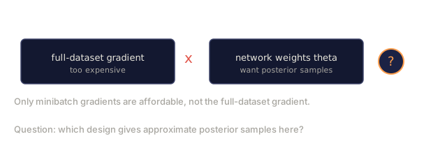
SGLD (Stochastic Gradient Langevin Dynamics) combines mini-batch gradient descent with Langevin noise: instead of computing the full gradient, you use a stochastic estimate and add calibrated noise on top. As the learning rate decays, SGLD drifts from optimization toward sampling, and you end up with approximate Bayesian posterior samples for free. It's one of the simplest ways to pull uncertainty estimates out of a neural network.
The thread running through all of this: stochastic processes aren't just theory you learn once and forget. They're the actual computational mechanism running inside modern AI systems. Tune an LLM's temperature and you're adjusting a Markov chain. Train a diffusion model and you're learning to reverse a Brownian-motion-like process. Run Bayesian inference and you're constructing a chain that converges to the posterior.
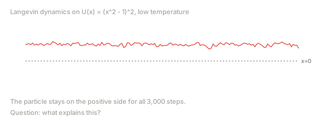
MCMC's convergence guarantee is real, but it's asymptotic: given infinite time, the chain samples from p(x) exactly. In finite time, on a genuinely multimodal target, that guarantee buys less than the Concept section's confident tone suggests. Run Exercise 4's double-well potential U(x) = (x^2 - 1)^2 at a temperature low enough to keep samples pinned near one well, and both Metropolis-Hastings and Langevin dynamics can spend thousands of steps orbiting that well before ever crossing to the other one. The acceptance ratio has no way to know the second well exists until a proposal happens to reach across the gap. This is exactly why practitioners run multiple chains from different starting points and check they agree: a single chain that looks perfectly converged can just be very good at exploring half the distribution.
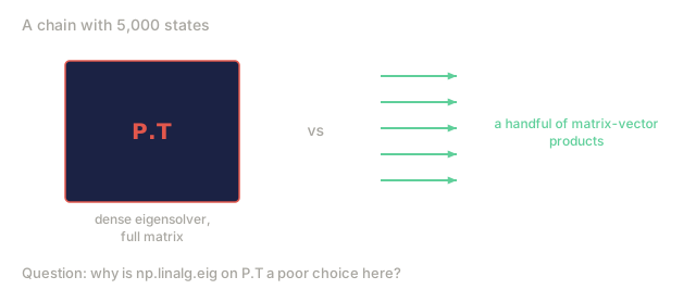
One more thing I'd flag: MarkovChain.stationary_distribution above calls np.linalg.eig on the full P^T and searches for the eigenvalue closest to 1. That's correct, and it's fine for a 3-state weather chain. It's also a dense, general-purpose eigensolver doing O(n^3) work to answer a question the power method, covered right above it, answers with a handful of matrix-vector products. Past a few hundred states, reach for the power method or a sparse solver instead of eig.
Exercises
-
Simulate 1000 random walks of 10000 steps each. Plot the distribution of final positions and verify it's approximately Gaussian with mean 0 and standard deviation sqrt(10000) = 100.
-
Build a text generator using a Markov chain. Train it on a small corpus: for each word, count transitions to the next word, build the transition matrix, then generate new sentences by sampling from the chain.
-
Implement simulated annealing using Metropolis-Hastings. Start at high temperature, where almost everything gets accepted, then cool down gradually until only improvements are accepted. Use it to find the minimum of a function with many local minima.
-
Compare Langevin dynamics at different temperatures. Sample from a double-well potential U(x) = (x^2 - 1)^2. At low temperature, samples cluster in one well; at high temperature, they spread across both. Find the critical temperature where the chain starts mixing between wells.
-
Implement the forward diffusion process. Start with a 1D signal, like a sine wave, and add noise progressively over 100 steps with a linear noise schedule. Show how the signal degrades to pure noise, then implement a simple denoiser that reverses the process, even a naive one that just subtracts the estimated noise.
Key Terms
| Term | What people say | What it actually means |
|---|---|---|
| Random walk | "Coin-flip movement" | A process where position changes by random increments at each step |
| Markov property | "Memoryless" | The future depends only on the present state, not on the history |
| Transition matrix | "The probability table" | P[i][j] = probability of moving from state i to state j |
| Stationary distribution | "The long-run average" | The distribution pi where pi*P = pi -- the chain's equilibrium |
| Brownian motion | "Random jiggling" | The continuous-time limit of a random walk, B(t) ~ N(0, t) |
| Langevin dynamics | "Gradient descent with noise" | Update rule that combines deterministic gradient and random perturbation |
| MCMC | "Walking toward the target" | Constructing a Markov chain whose stationary distribution is the one you want |
| Metropolis-Hastings | "Propose and accept/reject" | MCMC algorithm that uses acceptance ratios to ensure convergence |
| Temperature | "The randomness knob" | Parameter controlling the tradeoff between exploration and exploitation |
| Diffusion process | "Noise in, noise out" | Forward: gradually add noise. Reverse: gradually remove it. Generates data. |
Further Reading
- Ho, Jain, Abbeel (2020): "Denoising Diffusion Probabilistic Models." The DDPM paper that launched the diffusion model revolution, with a clear derivation of the forward and reverse Markov chains.
- Song & Ermon (2019): "Generative Modeling by Estimating Gradients of the Data Distribution." The score-based approach to sampling, built on Langevin dynamics.
- Roberts & Rosenthal (2004): "General state space Markov chains and MCMC algorithms." The theory behind when and why MCMC actually works.
- Norris (1997): "Markov Chains." The standard textbook, covering convergence, stationary distributions, and hitting times.
- Welling & Teh (2011): "Bayesian Learning via Stochastic Gradient Langevin Dynamics." Combines SGD with Langevin dynamics for scalable Bayesian inference.
Code
- stochastic.py (python, 277 lines)