Graph Theory for Machine Learning
Graphs are the data structure of relationships. The moment your data has connections, tables stop being enough.
Learning Objectives
- Build a graph class with adjacency matrix/list representations and implement BFS and DFS traversals
- Compute the graph Laplacian and use its eigenvalues to detect connected components and cluster nodes
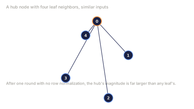
- Implement one round of GNN-style message passing as a normalized adjacency matrix multiplication
- Apply spectral clustering to partition a graph using the Fiedler vector
The Problem
Social networks, molecules, knowledge bases, citation networks, road maps: all of them are graphs. Traditional ML treats data as flat tables, where each row stands alone and each feature is a column. That works fine until the structure of the connections is the point, and then tables fail.
Take a social network. You want to predict what a user buys next. Their own purchase history matters, but their friends' history matters more: the connections carry signal that no single row captures.
Or take a molecule. You want to predict whether it binds to a protein. The atoms matter, but what actually determines binding is how those atoms are bonded to each other. The structure is the data, not a property sitting alongside it.
Graph Neural Networks (GNNs) are the fastest-growing area in deep learning. They power drug discovery, social recommendation, fraud detection, and knowledge graph reasoning. Every GNN builds on the same foundation: basic graph theory.
You need four things:
- A way to represent graphs as matrices (so you can multiply them)
- Traversal algorithms to explore graph structure
- The Laplacian, the single most important matrix in spectral graph theory
- Message passing, the operation that makes GNNs work
The Concept
Graphs: Nodes and Edges
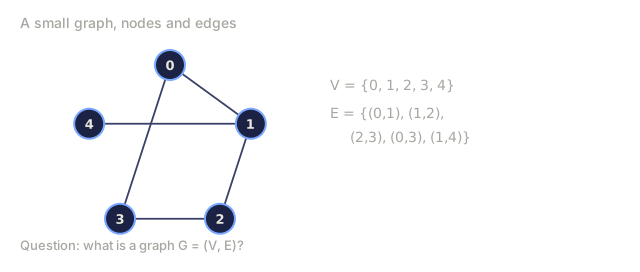
A graph G = (V, E) consists of vertices (nodes) V and edges E, where each edge connects two nodes.
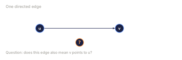
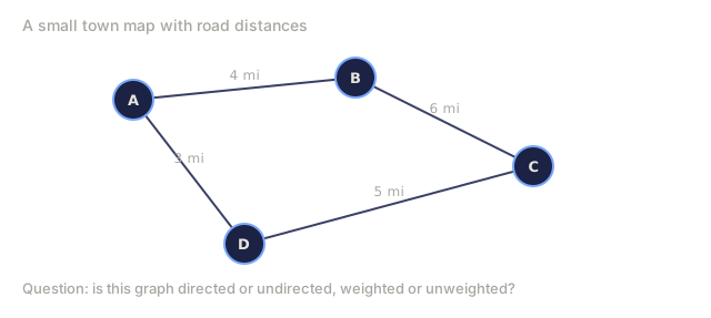
Directed vs undirected. In an undirected graph, edge (u, v) means u connects to v and v connects to u. In a directed graph (a digraph), edge (u, v) means u points to v, not necessarily the reverse.
Weighted vs unweighted. In an unweighted graph, edges simply exist or they don't. In a weighted graph, each edge carries a numerical weight: a distance, a cost, a strength.
| Graph type | Example |
|---|---|
| Undirected, unweighted | Facebook friendship network |
| Directed, unweighted | Twitter follow network |
| Undirected, weighted | Road map (distances) |
| Directed, weighted | Web page links (PageRank scores) |
The Adjacency Matrix
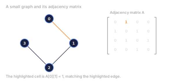
The adjacency matrix A is the core representation of a graph. For a graph with n nodes:
A[i][j] = 1    if there is an edge from node i to node j
A[i][j] = 0    otherwise
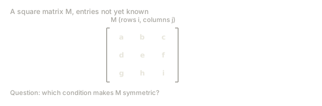
For undirected graphs, A is symmetric: A[i][j] = A[j][i]. For weighted graphs, A[i][j] holds the weight of edge (i, j).
Example: a triangle
Nodes: 0, 1, 2
Edges: (0,1), (1,2), (0,2)

A = [[0, 1, 1],
     [1, 0, 1],
     [1, 1, 0]]
The adjacency matrix is the input to every GNN, and matrix operations on A correspond directly to operations on the graph.
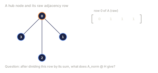
Analogy: an adjacency matrix is a seating chart turned into a grid. Row i lists everyone person i is connected to, one column per possible connection, so reading across a row tells you that node's entire neighborhood in one line.
Degree
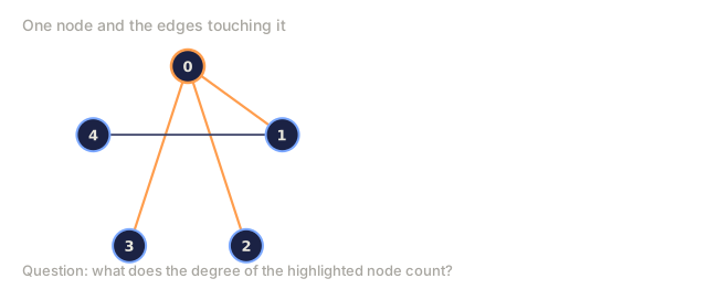
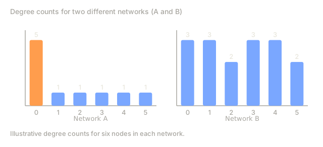
The degree of a node is the number of edges touching it. For directed graphs, you get in-degree (edges coming in) and out-degree (edges going out).
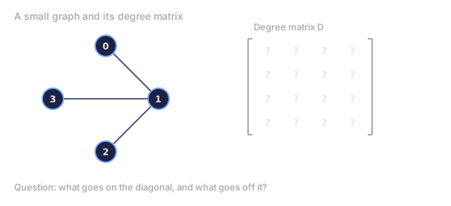
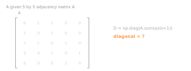
The degree matrix D is diagonal:
D[i][i] = degree of node i
D[i][j] = 0    for i != j
For the triangle example: D = diag(2, 2, 2), because every node connects to two others.
Degree tells you about node importance. High degree means a hub node. The degree distribution of a network reveals its structure: social networks follow power laws (few hubs, many leaf nodes), while random graphs have Poisson-distributed degrees, clustered tightly around one average with no real hubs at all.
Analogy: degree is a popularity count, how many other nodes are directly connected to you. It says nothing about the connections two hops away, which is exactly why BFS and DFS exist: to see past what one node's degree can tell you.
BFS and DFS
There are two fundamental graph traversal algorithms, and you need both.
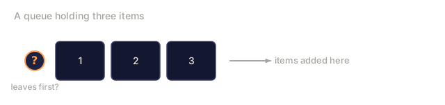
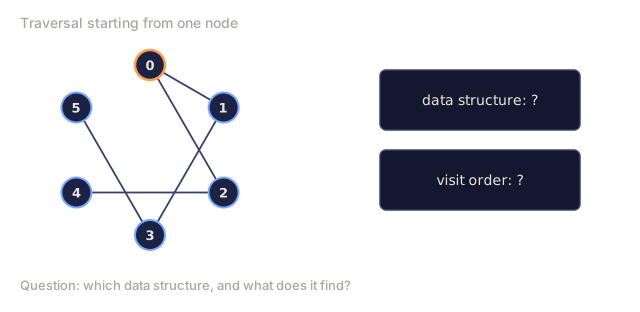
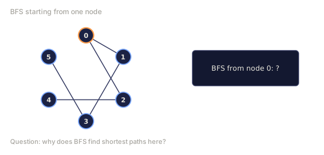
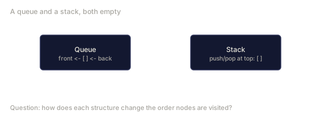
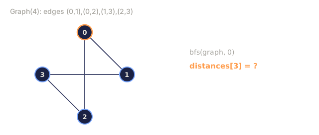
Breadth-First Search (BFS): explore all neighbors first, then neighbors' neighbors, using a queue (FIFO).
BFS from node 0:
  Visit 0
  Queue: [1, 2]        (neighbors of 0)
  Visit 1
  Queue: [2, 3]        (add neighbors of 1)
  Visit 2
  Queue: [3]           (neighbors of 2 already visited)
  Visit 3
  Queue: []            (done)
BFS finds shortest paths in unweighted graphs. The distance from the start to any node equals the BFS level at which that node is first discovered, which is why BFS is the standard tool for hop-count distances in social networks.
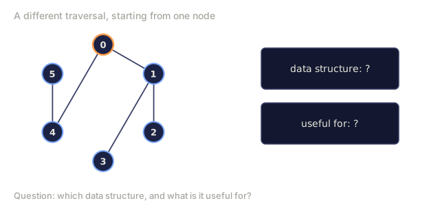
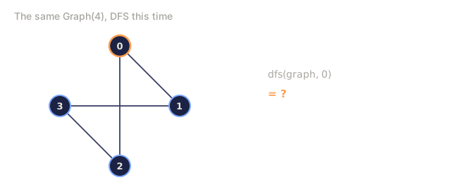
Depth-First Search (DFS): go as deep as possible before backtracking, using a stack (LIFO) or recursion.
DFS from node 0:
  Visit 0
  Stack: [1, 2]        (neighbors of 0)
  Visit 2               (pop from stack)
  Stack: [1, 3]         (add neighbors of 2)
  Visit 3               (pop from stack)
  Stack: [1]
  Visit 1               (pop from stack)
  Stack: []             (done)
DFS is useful for:
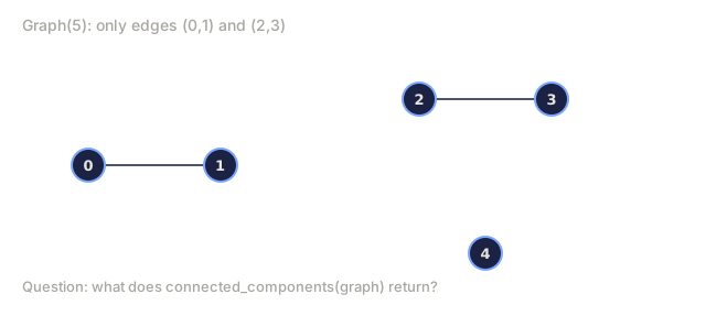
- Finding connected components (run DFS from unvisited nodes)
- Cycle detection (back edges in DFS tree)
- Topological sorting (reverse DFS finish order)
| Algorithm | Data structure | Finds | Use case |
|---|---|---|---|
| BFS | Queue | Shortest paths | Social network distance, knowledge graph traversal |
| DFS | Stack | Components, cycles | Connectivity, topological sort |
The Graph Laplacian
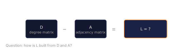
L = D - A: the single most important matrix in spectral graph theory.
For the triangle:
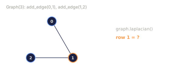
D = [[2, 0, 0],    A = [[0, 1, 1],    L = [[2, -1, -1],
     [0, 2, 0],         [1, 0, 1],         [-1, 2, -1],
     [0, 0, 2]]         [1, 1, 0]]         [-1, -1,  2]]
The Laplacian has remarkable properties:
-
L is positive semi-definite. All eigenvalues are >= 0.
-
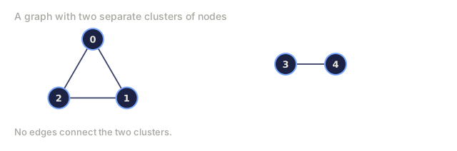
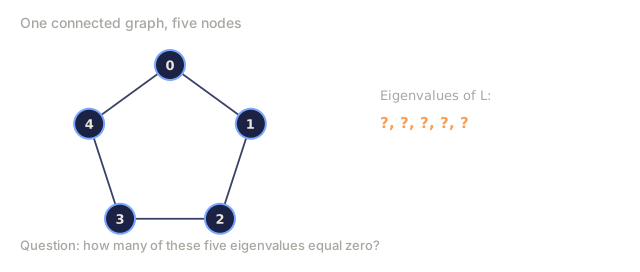
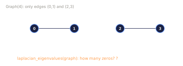
The number of zero eigenvalues equals the number of connected components (maximal groups of nodes that can all reach each other). A connected graph has exactly one zero eigenvalue. A graph with 3 disconnected components has three zero eigenvalues.
-
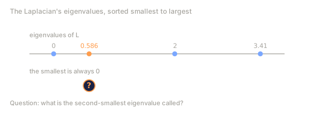
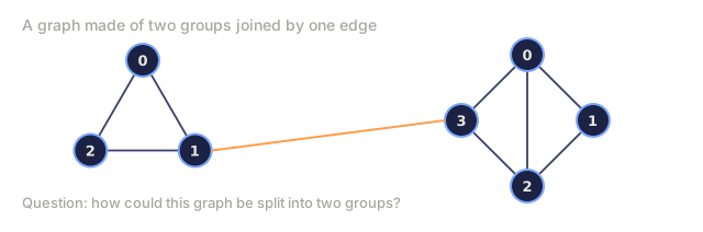
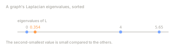
The smallest non-zero eigenvalue (Fiedler value) measures connectivity. A large Fiedler value means the graph is well-connected. A small one means the graph has a weak point: a bottleneck.
-
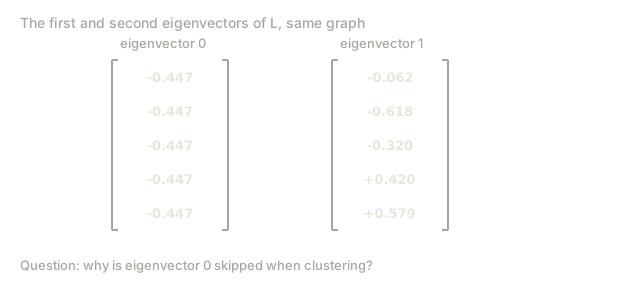
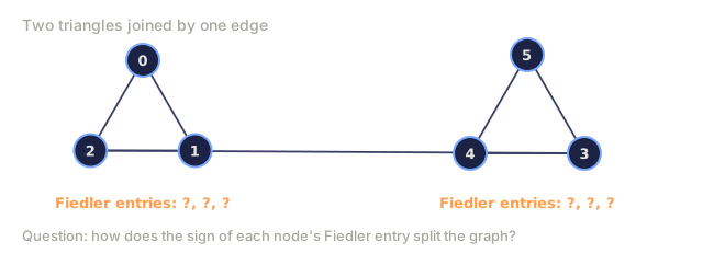
The eigenvector of the Fiedler value (Fiedler vector) reveals the best split. Nodes with positive values go in one group, nodes with negative values go in the other. This is spectral clustering.
Analogy: picture the Laplacian as a thermostat check. For every node, it compares that node's value to the average of its neighbors. A well-connected graph evens out fast; a graph with a weak point stays lopsided right there, which is exactly what a small Fiedler value flags.

Spectral Properties
The eigenvalues of the adjacency matrix and Laplacian reveal structural properties without any traversal at all.
Spectral clustering works like this:
- Compute the Laplacian L
- Find the k smallest eigenvectors of L (skip the first, which is all-ones for connected graphs)
- Use those eigenvectors as new coordinates for each node
- Run k-means on those coordinates
Why does this work? The eigenvectors of L encode the "smoothest" functions on the graph. Nodes that are well-connected get similar eigenvector values, while nodes separated by a bottleneck get very different ones. The eigenvectors naturally separate clusters.
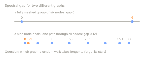
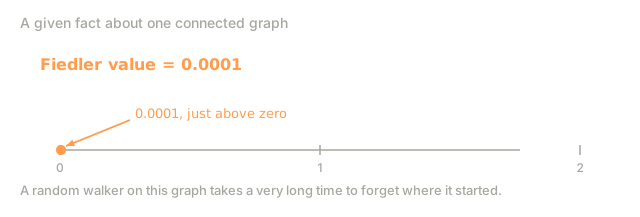
Random walk connection. The normalized Laplacian relates to random walks on the graph: the stationary distribution of a random walk is proportional to node degree, and the mixing time (how fast the walk converges) depends on the spectral gap, the same Fiedler value from before. A well-connected graph mixes fast: a random walker forgets where it started after a few steps. A graph with a bottleneck mixes slowly, which is exactly the graph shape the Fiedler value already flagged as weakly connected.
PageRank puts that random walk to work. Picture a surfer who follows a random outgoing link with probability d = 0.85 and otherwise jumps to a uniformly random node. A node's score is the share of time the surfer spends on it in the long run, so a node scores high when many nodes point to it, especially nodes that score high themselves. You compute it by iterating score(v) = (1-d)/n + d * sum(score(u)/out_degree(u)) over every u pointing to v, starting from uniform scores, until the scores stop changing. A node with no outgoing edges spreads its score evenly over all n nodes.
Message Passing
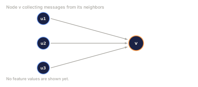
Message passing is the core operation of Graph Neural Networks: each node collects messages from its neighbors, aggregates them, and updates its own state.
h_v^(k+1) = UPDATE(h_v^(k), AGGREGATE({h_u^(k) : u in neighbors(v)}))
In the simplest form, AGGREGATE = mean, and UPDATE = linear transform + activation:
h_v^(k+1) = sigma(W * mean({h_u^(k) : u in neighbors(v)}))
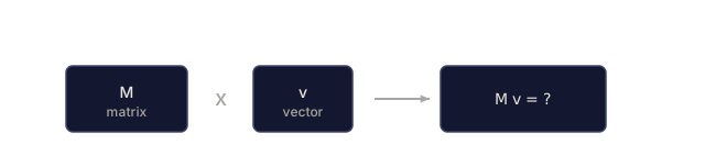
This is matrix multiplication in disguise. If H is the matrix of all node features and A is the adjacency matrix:
H^(k+1) = sigma(A_norm * H^(k) * W)
where A_norm is the normalized adjacency matrix (each row sums to 1).
Analogy: message passing is a rumor spreading at a party. Each round, you update your opinion to match the average opinion of whoever you're currently talking to. After enough rounds, opinions from across the whole room have filtered down to you, one conversation at a time.
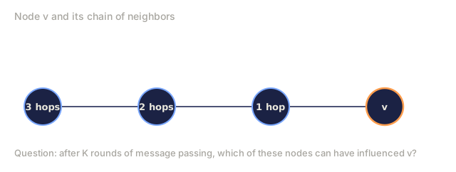
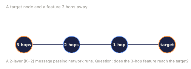
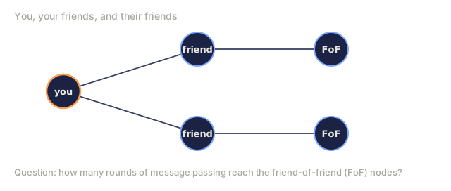
One round of message passing lets each node "see" its immediate neighbors. Two rounds let it see neighbors of neighbors. K rounds give each node information from its K-hop neighborhood.

Concepts and ML Applications
| Concept | ML Application |
|---|---|
| Adjacency matrix | GNN input representation |
| Graph Laplacian | Spectral clustering, community detection |
| BFS/DFS | Knowledge graph traversal, path finding |
| Degree distribution | Node importance, feature engineering |
| Message passing | GNN layers (GCN, GAT, GraphSAGE) |
| Eigenvalues of L | Community detection, graph partitioning |
| Spectral clustering | Unsupervised node grouping |
| PageRank | Node importance, web search |
Build It
Step 1: Graph class from scratch
class Graph:
    def __init__(self, n_nodes, directed=False):
        self.n = n_nodes
        self.directed = directed
        self.adj = {i: {} for i in range(n_nodes)}

    def add_edge(self, u, v, weight=1.0):
        self.adj[u][v] = weight
        if not self.directed:
            self.adj[v][u] = weight

    def neighbors(self, node):
        return list(self.adj[node].keys())

    def degree(self, node):
        return len(self.adj[node])

    def adjacency_matrix(self):
        import numpy as np
        A = np.zeros((self.n, self.n))
        for u in range(self.n):
            for v, w in self.adj[u].items():
                A[u][v] = w
        return A

    def degree_matrix(self):
        import numpy as np
        D = np.zeros((self.n, self.n))
        for i in range(self.n):
            D[i][i] = self.degree(i)
        return D

    def laplacian(self):
        return self.degree_matrix() - self.adjacency_matrix()
The adjacency list (self.adj) stores neighbors efficiently. The adjacency matrix conversion uses numpy, since all the spectral operations need it.
Step 2: BFS and DFS
from collections import deque

def bfs(graph, start):
    visited = set()
    order = []
    distances = {}
    queue = deque([(start, 0)])
    visited.add(start)
    while queue:
        node, dist = queue.popleft()
        order.append(node)
        distances[node] = dist
        for neighbor in graph.neighbors(node):
            if neighbor not in visited:
                visited.add(neighbor)
                queue.append((neighbor, dist + 1))
    return order, distances


def dfs(graph, start):
    visited = set()
    order = []
    stack = [start]
    while stack:
        node = stack.pop()
        if node in visited:
            continue
        visited.add(node)
        order.append(node)
        for neighbor in reversed(graph.neighbors(node)):
            if neighbor not in visited:
                stack.append(neighbor)
    return order
BFS uses a deque (double-ended queue) for O(1) popleft. DFS uses a list as a stack. Both visit every node exactly once, for O(V + E) time.
Step 3: Connected components and Laplacian eigenvalues
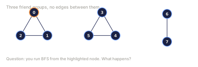
def connected_components(graph):
    visited = set()
    components = []
    for node in range(graph.n):
        if node not in visited:
            order, _ = bfs(graph, node)
            visited.update(order)
            components.append(order)
    return components


def laplacian_eigenvalues(graph):
    import numpy as np
    L = graph.laplacian()
    eigenvalues = np.linalg.eigvalsh(L)
    return eigenvalues
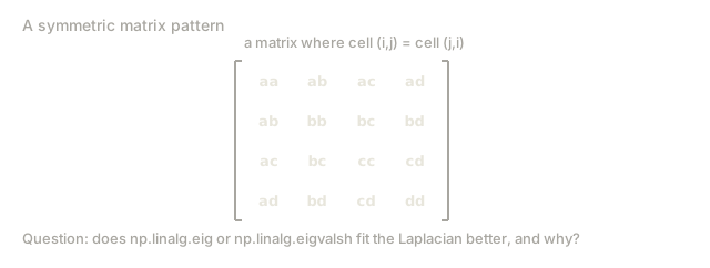
eigvalsh is for symmetric matrices, and the Laplacian is always symmetric for undirected graphs. It returns eigenvalues in ascending order, so counting the zeros tells you the number of connected components.
Step 4: Spectral clustering
def spectral_clustering(graph, k=2):
    import numpy as np
    L = graph.laplacian()
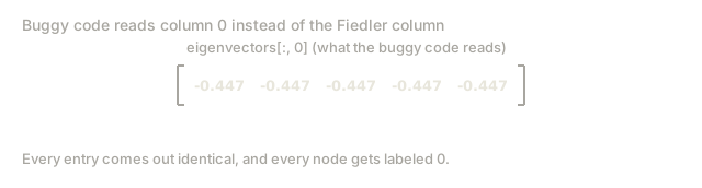
    eigenvalues, eigenvectors = np.linalg.eigh(L)
    features = eigenvectors[:, 1:k+1]

    labels = np.zeros(graph.n, dtype=int)
    for i in range(graph.n):
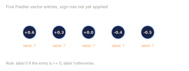
        if features[i, 0] >= 0:
            labels[i] = 0
        else:
            labels[i] = 1
    return labels
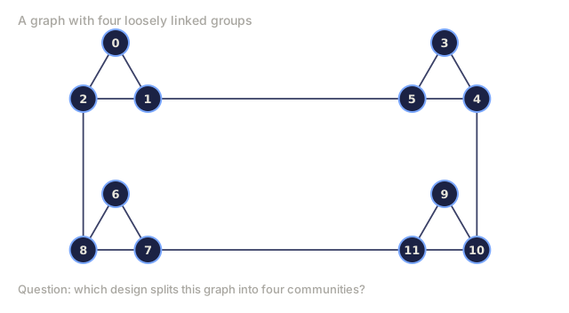
For k=2, the sign of the Fiedler vector splits the graph into two clusters. For k>2, run k-means on the first k eigenvectors instead (excluding the trivial all-ones eigenvector).
Step 5: Message passing
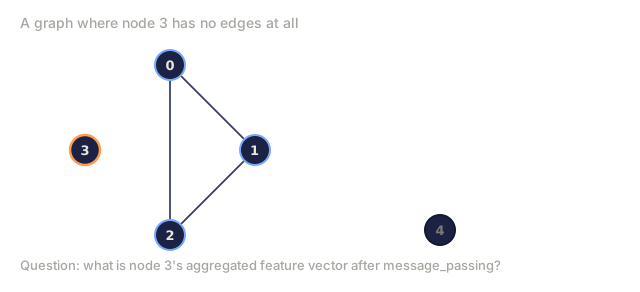
def message_passing(graph, features, weight_matrix):
    import numpy as np
    A = graph.adjacency_matrix()
    row_sums = A.sum(axis=1, keepdims=True)
    row_sums[row_sums == 0] = 1
    A_norm = A / row_sums
    aggregated = A_norm @ features
    output = aggregated @ weight_matrix
    return output
This is one round of GNN message passing: each node's new features are the weighted average of its neighbors' features, transformed by the weight matrix. Stack multiple rounds to propagate information further.
Use It
With networkx and numpy, the same operations are one-liners:
import networkx as nx
import numpy as np

G = nx.karate_club_graph()

A = nx.adjacency_matrix(G).toarray()
L = nx.laplacian_matrix(G).toarray()

eigenvalues = np.linalg.eigvalsh(L.astype(float))
print(f"Smallest eigenvalues: {eigenvalues[:5]}")
print(f"Connected components: {nx.number_connected_components(G)}")

communities = nx.community.greedy_modularity_communities(G)
print(f"Communities found: {len(communities)}")

pr = nx.pagerank(G)
top_nodes = sorted(pr.items(), key=lambda x: x[1], reverse=True)[:5]
print(f"Top 5 PageRank nodes: {top_nodes}")
networkx handles graphs of any size with optimized C backends. Use it in production. Use your from-scratch implementation to understand what it does.
numpy spectral analysis
import numpy as np

A = np.array([
    [0, 1, 1, 0, 0],
    [1, 0, 1, 0, 0],
    [1, 1, 0, 1, 0],
    [0, 0, 1, 0, 1],
    [0, 0, 0, 1, 0]
])

D = np.diag(A.sum(axis=1))
L = D - A

eigenvalues, eigenvectors = np.linalg.eigh(L)
print(f"Eigenvalues: {np.round(eigenvalues, 4)}")
print(f"Fiedler value: {eigenvalues[1]:.4f}")
print(f"Fiedler vector: {np.round(eigenvectors[:, 1], 4)}")

fiedler = eigenvectors[:, 1]
group_a = np.where(fiedler >= 0)[0]
group_b = np.where(fiedler < 0)[0]
print(f"Cluster A: {group_a}")
print(f"Cluster B: {group_b}")
The Fiedler vector does the heavy lifting: positive entries in one cluster, negative in the other. No iterative optimization needed, just one eigendecomposition.
Ship It
This lesson produces:
outputs/skill-graph-analysis.md, a skill reference for analyzing graph-structured data
Connections
| Concept | Where it shows up |
|---|---|
| Adjacency matrix | GCN, GAT, GraphSAGE input |
| Laplacian | Spectral clustering, ChebNet filters |
| BFS | Knowledge graph traversal, shortest path queries |
| Message passing | Every GNN layer, neural message passing |
| Spectral gap | Graph connectivity, mixing time of random walks |
| Degree distribution | Power-law networks, node feature engineering |
| Connected components | Preprocessing, handling disconnected graphs |
| PageRank | Node importance ranking, attention initialization |
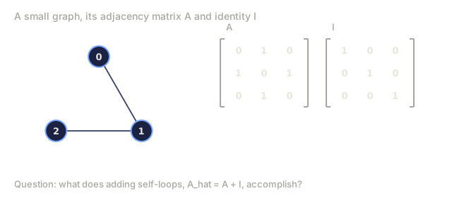
GNNs deserve special mention here. The graph convolution operation in GCN (Kipf & Welling, 2017) uses the adjacency matrix with added self-loops, A_hat = A + I:
H^(l+1) = sigma(D_hat^(-1/2) * A_hat * D_hat^(-1/2) * H^(l) * W^(l))where A_hat = A + I (adjacency plus self-loops) and D_hat is the degree matrix of A_hat. The self-loops ensure each node includes its own features during aggregation, not just its neighbors'. That's exactly message passing with symmetric normalization: D_hat^(-1/2) * A_hat * D_hat^(-1/2) is the normalized adjacency matrix. The Laplacian shows up here because this normalization is related to L_sym = I - D^(-1/2) * A * D^(-1/2), and understanding the Laplacian means understanding why GCNs actually work.
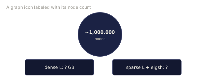
The eigendecomposition in this lesson runs on np.linalg.eigh, dense and exact, and that's fine for a triangle or the 34-node Karate Club graph. It stops being fine the moment you point it at anything with more than a few thousand nodes: a dense n x n Laplacian for a million-node graph needs on the order of 8 terabytes just to store the floats, before you've done a single flop of the O(n^3) eigendecomposition. In practice you reach for scipy.sparse.linalg.eigsh, which only computes the k eigenvectors you actually care about and exploits the fact that real graphs have far fewer edges than the n^2 a dense matrix assumes.
The other thing I'd flag: don't let the Karate Club example convince you spectral clustering is plug-and-play. It works cleanly there because the ground-truth split lines up with what a bisection of the Fiedler vector finds. Real graphs with more than two natural communities, or communities of wildly different sizes, need k > 2 eigenvectors and an actual k-means step, and the result is a lot more sensitive to how you normalize the Laplacian (D^(-1/2) L D^(-1/2) versus the raw L = D - A) than this lesson's code lets on. Try both on a graph you already know the answer for before trusting either on one you don't.
Exercises
-
Implement PageRank from scratch. Start with uniform scores. At each step: score(v) = (1-d)/n + d * sum(score(u)/out_degree(u)) for all u pointing to v. Use d=0.85. Run until convergence (change < 1e-6). Test on a small web graph.
-
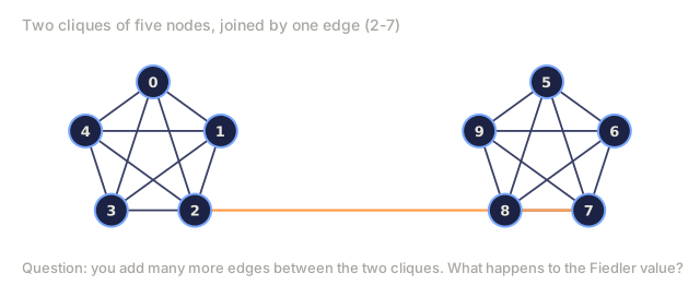
Find communities using spectral clustering. Create a graph with two clearly separated clusters (e.g., two cliques connected by a single edge). Run spectral clustering and verify it finds the right split. What happens as you add more cross-cluster edges?
-
Implement Dijkstra's algorithm for shortest paths in weighted graphs. Compare results to BFS on the same graph with uniform weights.
-
Build a 2-layer message passing network. Apply message passing twice with different weight matrices. Show that after 2 rounds, each node has information from its 2-hop neighborhood.
-
Analyze a real-world graph. Use the Karate Club graph (34 nodes, 78 edges). Compute degree distribution, Laplacian eigenvalues, and spectral clustering. Compare the spectral clustering result to the known ground truth split.
Key Terms
| Term | What people say | What it actually means |
|---|---|---|
| Graph | "Nodes and edges" | A mathematical structure G=(V,E) encoding pairwise relationships |
| Adjacency matrix | "The connection table" | An n x n matrix where A[i][j] = 1 if nodes i and j are connected |
| Degree | "How connected a node is" | The number of edges touching a node |
| Laplacian | "D minus A" | L = D - A, the matrix whose eigenvalues reveal graph structure |
| Fiedler value | "The algebraic connectivity" | The smallest non-zero eigenvalue of L, measuring how well-connected the graph is |
| BFS | "Level-by-level search" | Traversal that visits all neighbors before going deeper, finds shortest paths |
| DFS | "Go deep first" | Traversal that follows one path to its end before backtracking |
| Message passing | "Nodes talk to neighbors" | Each node aggregates information from its neighbors, the core of GNNs |
| Spectral clustering | "Cluster by eigenvectors" | Partition a graph using eigenvectors of its Laplacian |
| Connected component | "A separate piece" | A maximal subgraph where every node can reach every other node |
Further Reading
- Kipf & Welling (2017) — "Semi-Supervised Classification with Graph Convolutional Networks." The paper that launched modern GNNs, showing spectral graph convolutions simplify to message passing.
- Spielman (2012) — "Spectral Graph Theory" lecture notes. The definitive introduction to Laplacians, spectral gaps, and graph partitioning.
- Hamilton (2020) — "Graph Representation Learning." Covers GNNs from fundamentals through applications.
- Bronstein et al. (2021) — "Geometric Deep Learning: Grids, Groups, Graphs, Geodesics, and Gauges." The unifying framework paper.
- Veličković et al. (2018) — "Graph Attention Networks." Extends message passing with attention mechanisms.
Code
- graph_theory.py (python, 308 lines)