Backpropagation from Scratch
Backpropagation is what makes learning possible. Without it, a neural network is just an expensive random number generator.
Learning Objectives
- Implement a Value-based autograd engine that builds a computational graph and computes gradients via topological sort
- Derive the backward pass for addition, multiplication, and sigmoid using the chain rule
- Train a multi-layer network on XOR and circle classification using only your from-scratch backpropagation engine
- Identify the vanishing gradient problem in deep sigmoid networks and explain why gradients shrink exponentially
The Problem
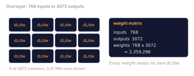
Take a network with a single hidden layer: 768 inputs, 3072 outputs. That's 2,359,296 weights. Say it makes a wrong prediction and you need to know which weights caused the error. Testing each weight individually means running 2.3 million forward passes, one per weight, just to see how the loss moves. Backpropagation computes all 2.3 million gradients in a single backward pass instead. That isn't a minor speedup; it's the difference between a network you can train and one you can't.
The naive approach would be: nudge one weight by a tiny amount, rerun the forward pass, and check whether the loss went up or down. That gives you the gradient for that one weight. Now repeat it for every weight in the network, across thousands of training steps and millions of data points, and you'd need geological time to train anything useful.
Backpropagation solves this with one forward pass and one backward pass, computing every gradient in that single backward pass. The mechanism is the chain rule from calculus, applied systematically across a computational graph. It's the algorithm that made deep learning practical; without it, we'd still be stuck on toy problems.
The Concept
The Chain Rule, Applied to Networks
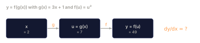
You saw the chain rule back in Phase 01, Lesson 05: if y = f(g(x)), then dy/dx = f'(g(x)) * g'(x). You multiply derivatives along the chain.
In a neural network, the "chain" is the sequence of operations from input to loss. Each layer applies weights, adds a bias, and passes the result through an activation function, and the loss function compares that final output to the target. Backpropagation traces the chain backward, computing how much each operation contributed to the error.
Computational Graphs
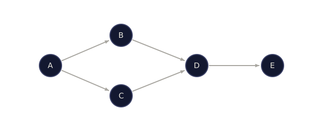
Every forward pass builds a graph. Each node is an operation, like multiply, add, or sigmoid, and each edge carries a value forward and a gradient backward.

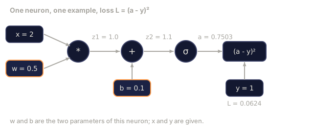
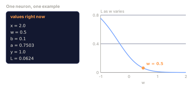
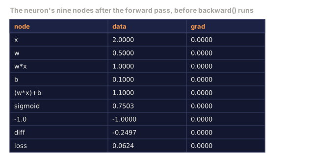
Forward pass: values flow left to right. x and w produce z1 = w*x. Add b to get z2. Sigmoid turns z2 into the activation a. Compare a to the target y with the loss function.
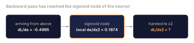
Backward pass: gradients flow right to left. Start with dL/da: how the loss changes with the activation. Multiply by da/dz2 (the sigmoid derivative) to get dL/dz2. That gradient splits two ways: dL/db, which equals dL/dz2 since z2 = z1 + b, and dL/dz1. From dL/dz1, dL/dw = dL/dz1 * x and dL/dx = dL/dz1 * w.
Every node in the graph has exactly one job during the backward pass: take the gradient coming from above, multiply it by its own local derivative, and pass the result down.
Forward vs Backward

The forward pass stores every intermediate value (z, a, the inputs to each layer) because the backward pass needs them to compute gradients. That's the memory-computation tradeoff at the heart of backprop: you trade memory (storing activations) for speed (one pass instead of millions).
Gradient Flow Through a Network
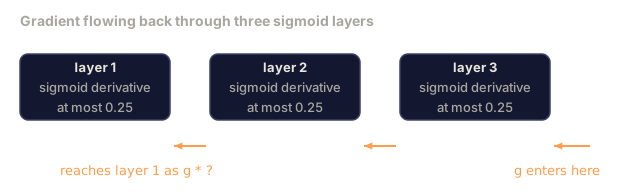
For a 3-layer network, gradients chain through every layer:

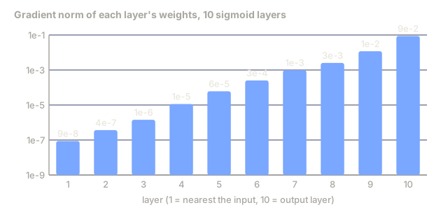
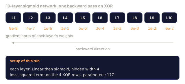
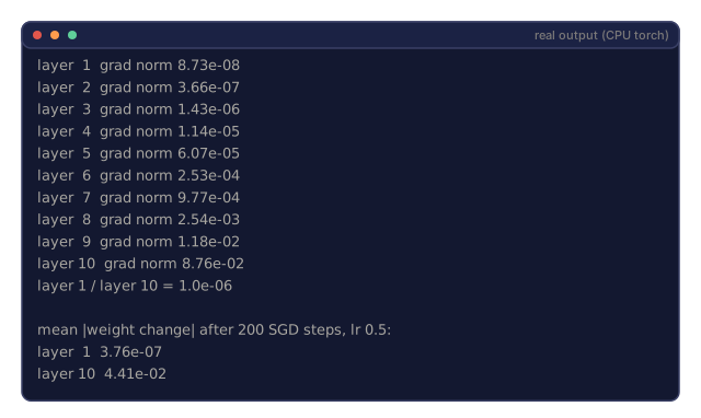
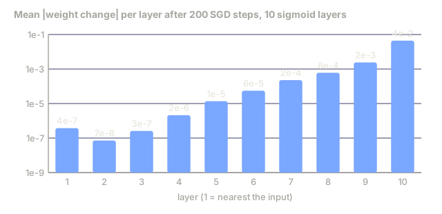
At each layer, the gradient gets multiplied by the sigmoid derivative, a * (1 - a), which maxes out at 0.25 when a = 0.5. Three layers deep, the gradient has been multiplied by at most 0.25^3 = 0.0156; ten layers deep, by 0.25^10 = 0.000001.
Vanishing Gradients
The vanishing gradient problem is this: sigmoid squashes its output between 0 and 1, its derivative never exceeds 0.25, and stacking enough sigmoid layers multiplies that small number by itself until the gradient shrinks to nothing. Early layers barely learn because they receive near-zero gradients.
sigmoid(z):     Output range [0, 1]
sigmoid'(z):    Max value 0.25 (at z = 0)

After 5 layers:   gradient * 0.25^5 = 0.001x original
After 10 layers:  gradient * 0.25^10 = 0.000001x original
This is why deep sigmoid networks are nearly impossible to train. The fix (ReLU and its variants) is the subject of Lesson 04. For now, understand that backprop itself works perfectly; the problem is what it's working through.
Deriving Gradients for a 2-Layer Network
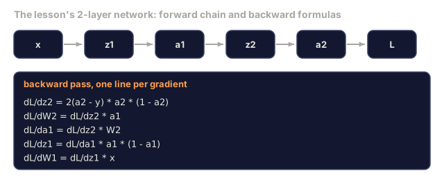
Here's the concrete math for a network with input x, a sigmoid hidden layer, a sigmoid output layer, and MSE loss.
Forward pass:
z1 = W1 * x + b1
a1 = sigmoid(z1)
z2 = W2 * a1 + b2
a2 = sigmoid(z2)
L = (a2 - y)^2
Backward pass (applying chain rule step by step):
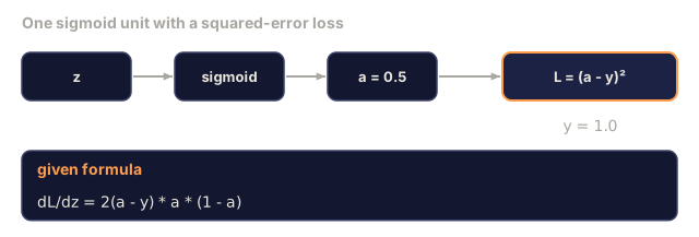
dL/da2 = 2(a2 - y)
da2/dz2 = a2 * (1 - a2)
dL/dz2 = dL/da2 * da2/dz2 = 2(a2 - y) * a2 * (1 - a2)

dL/dW2 = dL/dz2 * a1
dL/db2 = dL/dz2

dL/da1 = dL/dz2 * W2
da1/dz1 = a1 * (1 - a1)
dL/dz1 = dL/da1 * da1/dz1

dL/dW1 = dL/dz1 * x
dL/db1 = dL/dz1
Every gradient is a product of local derivatives traced back from the loss. That's all backpropagation is.
Build It
Step 1: The Value Node
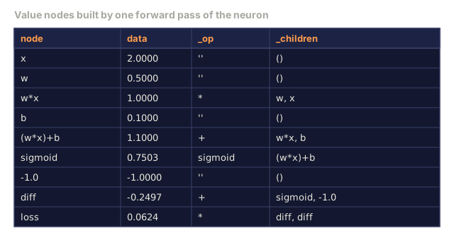
Every number in our computation becomes a Value. It stores its data, its gradient, and how it was created (so it knows how to compute gradients backward).
class Value:
    def __init__(self, data, children=(), op=''):
        self.data = data
        self.grad = 0.0
        self._backward = lambda: None
        self._children = set(children)
        self._op = op

    def __repr__(self):
        return f"Value(data={self.data:.4f}, grad={self.grad:.4f})"
There's no gradient yet (0.0) and no backward function yet (a no-op). The _children set tracks which Values produced this one, which is what lets us topologically sort the graph later.
Step 2: Operations with Backward Functions
Each operation creates a new Value and defines how gradients flow backward through it.
def __add__(self, other):
    other = other if isinstance(other, Value) else Value(other)
    out = Value(self.data + other.data, (self, other), '+')

    def _backward():
        self.grad += out.grad
        other.grad += out.grad

    out._backward = _backward
    return out

def __mul__(self, other):
    other = other if isinstance(other, Value) else Value(other)
    out = Value(self.data * other.data, (self, other), '*')

    def _backward():
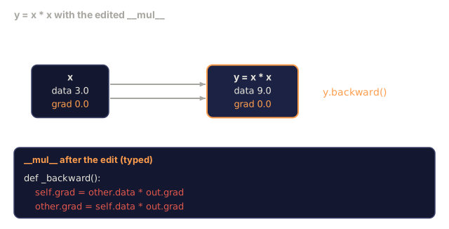
        self.grad += other.data * out.grad
        other.grad += self.data * out.grad

    out._backward = _backward
    return out
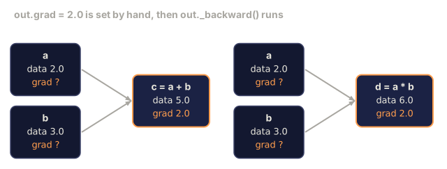
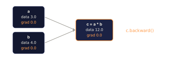
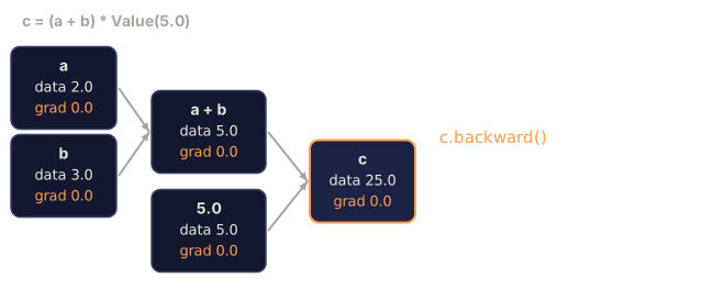
For addition, d(a+b)/da = 1 and d(a+b)/db = 1, so both inputs get the output's gradient directly. For multiplication, d(ab)/da = b and d(ab)/db = a, so each input gets the other's value times the output gradient.
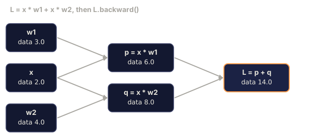
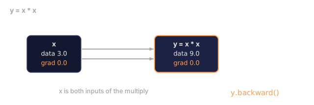
The += here is critical: a Value might be used in multiple operations, and its gradient is the sum of gradients from every path that uses it.
Step 3: Sigmoid and Loss
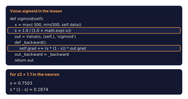
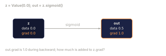
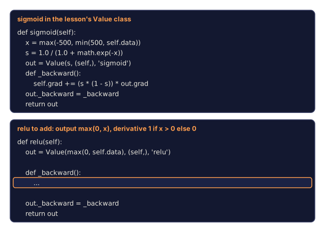
The sigmoid derivative is sigmoid(x) * (1 - sigmoid(x)). We already computed sigmoid(x) = s during the forward pass, so the backward function should just reuse it instead of recomputing anything:
import math

def sigmoid(self):
    x = self.data
    x = max(-500, min(500, x))
    s = 1.0 / (1.0 + math.exp(-x))
    out = Value(s, (self,), 'sigmoid')

    def _backward():
        self.grad += (s * (1 - s)) * out.grad

    out._backward = _backward
    return out
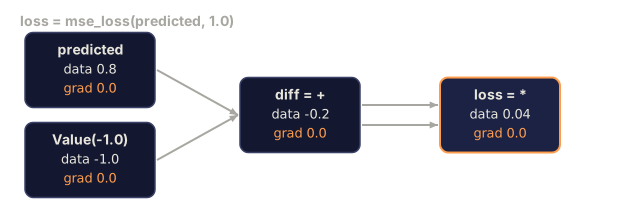
To train on XOR you'll need a single scalar to call .backward() on. MSE for one output is (predicted - target)^2, and we can express the subtraction as addition with a negated Value:
def mse_loss(predicted, target):
    diff = predicted + Value(-target)
    return diff * diff
Step 4: Backward Pass
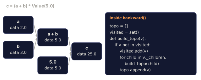
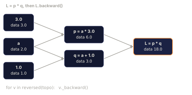
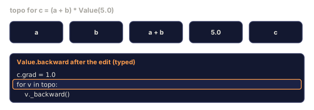
Topological sort ensures we process nodes in the right order: a node's gradient has to be fully accumulated before we propagate through it.
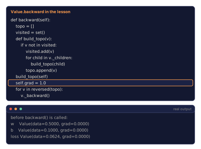
def backward(self):
    topo = []
    visited = set()

    def build_topo(v):
        if v not in visited:
            visited.add(v)
            for child in v._children:
                build_topo(child)
            topo.append(v)

    build_topo(self)
    self.grad = 1.0
    for v in reversed(topo):
        v._backward()
Start at the loss, with gradient 1.0 since dL/dL = 1, then walk backward through the sorted graph: each node's _backward pushes gradients to its children.
Step 5: Layer and Network
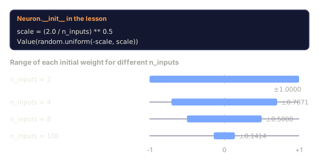
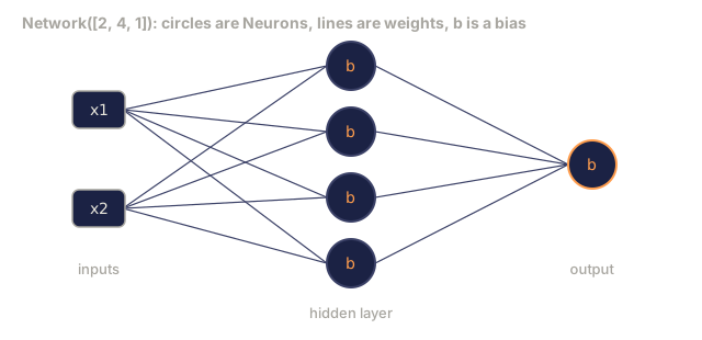
A Neuron needs to take inputs, compute a weighted sum plus bias, and apply sigmoid to it, exactly like the Value operations above but wired together into one unit. Its weight initialization scales by sqrt(2/n_inputs) to prevent sigmoid saturation in deeper networks. A Layer is a list of Neurons, and a Network is a list of Layers; the parameters() method on each collects every learnable Value so the training loop can update them later.
import random

class Neuron:
    def __init__(self, n_inputs):
        scale = (2.0 / n_inputs) ** 0.5
        self.weights = [Value(random.uniform(-scale, scale)) for _ in range(n_inputs)]
        self.bias = Value(0.0)

    def __call__(self, x):
        act = sum((wi * xi for wi, xi in zip(self.weights, x)), self.bias)
        return act.sigmoid()

    def parameters(self):
        return self.weights + [self.bias]


class Layer:
    def __init__(self, n_inputs, n_outputs):
        self.neurons = [Neuron(n_inputs) for _ in range(n_outputs)]

    def __call__(self, x):
        out = [n(x) for n in self.neurons]
        return out[0] if len(out) == 1 else out

    def parameters(self):
        params = []
        for n in self.neurons:
            params.extend(n.parameters())
        return params


class Network:
    def __init__(self, sizes):
        self.layers = []
        for i in range(len(sizes) - 1):
            self.layers.append(Layer(sizes[i], sizes[i + 1]))

    def __call__(self, x):
        for layer in self.layers:
            x = layer(x)
            if not isinstance(x, list):
                x = [x]
        return x[0] if len(x) == 1 else x

    def parameters(self):
        params = []
        for layer in self.layers:
            params.extend(layer.parameters())
        return params

    def zero_grad(self):
        for p in self.parameters():
            p.grad = 0.0
Step 6: Train on XOR
random.seed(42)
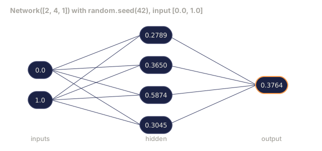
net = Network([2, 4, 1])

xor_data = [
    ([0.0, 0.0], 0.0),
    ([0.0, 1.0], 1.0),
    ([1.0, 0.0], 1.0),
    ([1.0, 1.0], 0.0),
]

learning_rate = 1.0

for epoch in range(1000):
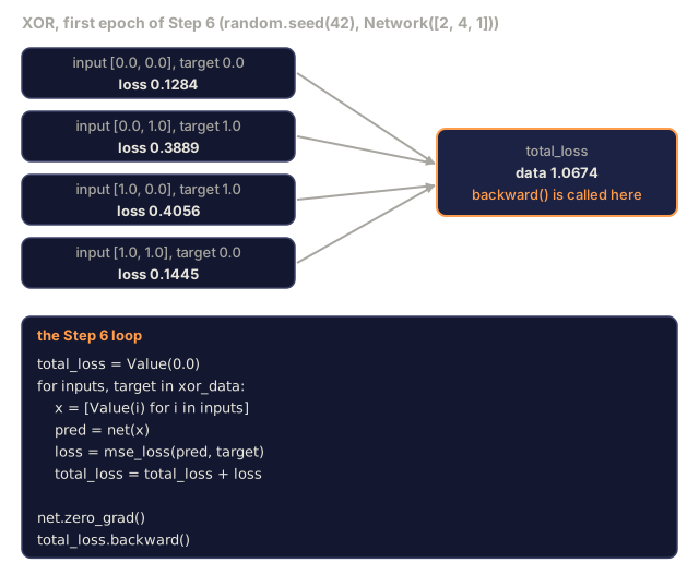
    total_loss = Value(0.0)
    for inputs, target in xor_data:
        x = [Value(i) for i in inputs]
        pred = net(x)
        loss = mse_loss(pred, target)
        total_loss = total_loss + loss

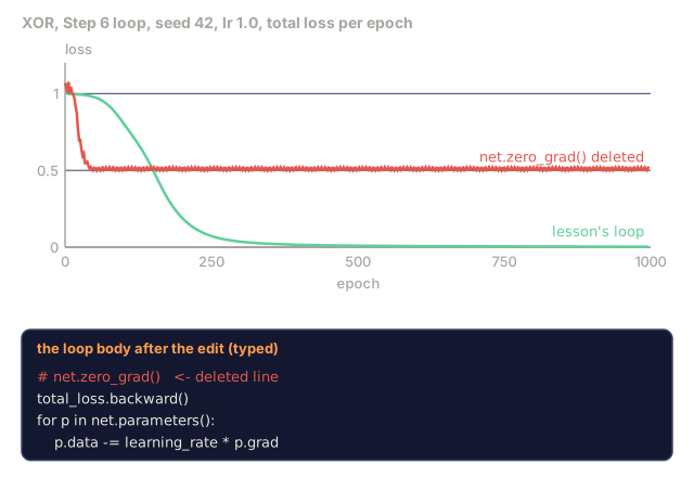
    net.zero_grad()
    total_loss.backward()

    for p in net.parameters():
        p.data -= learning_rate * p.grad

    if epoch % 100 == 0:
        print(f"Epoch {epoch:4d} | Loss: {total_loss.data:.6f}")

print("\nXOR Results:")
for inputs, target in xor_data:
    x = [Value(i) for i in inputs]
    pred = net(x)
    print(f"  {inputs} -> {pred.data:.4f} (expected {target})")
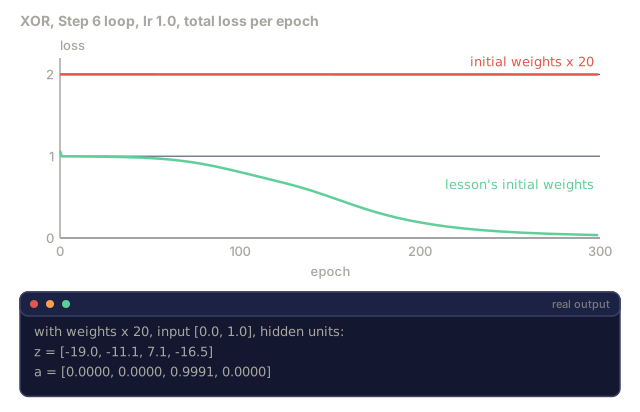
Watch the loss decrease: what starts as random predictions turns into correct XOR outputs, driven entirely by backpropagation computing gradients and nudging the weights in the right direction.
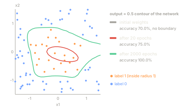
Step 7: Circle Classification
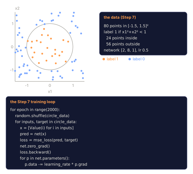
In Lesson 02, you hand-tuned weights for circle classification. Now let the network learn them.
random.seed(7)

def generate_circle_data(n=100):
    data = []
    for _ in range(n):
        x1 = random.uniform(-1.5, 1.5)
        x2 = random.uniform(-1.5, 1.5)
        label = 1.0 if x1 * x1 + x2 * x2 < 1.0 else 0.0
        data.append(([x1, x2], label))
    return data

circle_data = generate_circle_data(80)

circle_net = Network([2, 8, 1])
learning_rate = 0.5

for epoch in range(2000):
    random.shuffle(circle_data)
    total_loss_val = 0.0
    for inputs, target in circle_data:
        x = [Value(i) for i in inputs]
        pred = circle_net(x)
        loss = mse_loss(pred, target)
        circle_net.zero_grad()
        loss.backward()
        for p in circle_net.parameters():
            p.data -= learning_rate * p.grad
        total_loss_val += loss.data

    if epoch % 200 == 0:
        correct = 0
        for inputs, target in circle_data:
            x = [Value(i) for i in inputs]
            pred = circle_net(x)
            predicted_class = 1.0 if pred.data > 0.5 else 0.0
            if predicted_class == target:
                correct += 1
        accuracy = correct / len(circle_data) * 100
        print(f"Epoch {epoch:4d} | Loss: {total_loss_val:.4f} | Accuracy: {accuracy:.1f}%")
We use online SGD here: updating weights after each sample instead of accumulating the full batch. This breaks symmetry faster and avoids sigmoid saturation on the full loss landscape. Shuffling the data each epoch keeps the network from memorizing the order it was trained in.
No hand-tuning. The network discovers the circular decision boundary on its own. That's the power of backpropagation: you define the architecture, the loss function, and the data. The algorithm figures out the weights.
Use It
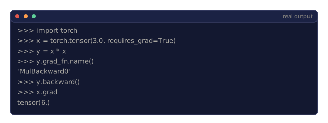
PyTorch does everything above in a few lines. The core idea is identical: autograd builds a computational graph during the forward pass and traces it backward to compute gradients.
import torch
import torch.nn as nn

model = nn.Sequential(
    nn.Linear(2, 4),
    nn.Sigmoid(),
    nn.Linear(4, 1),
    nn.Sigmoid(),
)
optimizer = torch.optim.SGD(model.parameters(), lr=1.0)
criterion = nn.MSELoss()

X = torch.tensor([[0,0],[0,1],[1,0],[1,1]], dtype=torch.float32)
y = torch.tensor([[0],[1],[1],[0]], dtype=torch.float32)

for epoch in range(1000):
    pred = model(X)
    loss = criterion(pred, y)
    optimizer.zero_grad()
    loss.backward()
    optimizer.step()

print("PyTorch XOR Results:")
with torch.no_grad():
    for i in range(4):
        pred = model(X[i])
        print(f"  {X[i].tolist()} -> {pred.item():.4f} (expected {y[i].item()})")
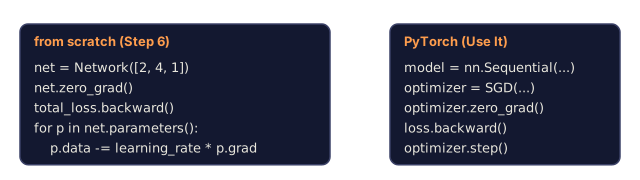
loss.backward() is your total_loss.backward(). optimizer.step() is your manual p.data -= lr * p.grad. optimizer.zero_grad() is your net.zero_grad(). Same algorithm, an industrial-strength implementation: PyTorch handles GPU acceleration, mixed precision, gradient checkpointing, and hundreds of layer types, but the backward pass is still the same chain rule applied to the same computational graph.
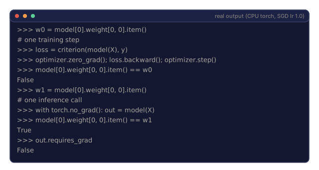
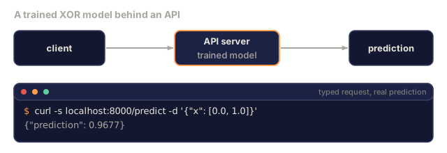
Training runs the forward pass, then the backward pass, then updates the weights. Inference runs only the forward pass: no gradients, no updates. That distinction matters because inference is what happens in production. When you call an API like Claude or GPT, you're running inference: your prompt flows forward through the network and tokens come out the other end, but no weights change. Understanding backprop matters because it shaped every weight in that network.
Ship It
This lesson produces:
outputs/prompt-gradient-debugger.md: a reusable prompt for diagnosing gradient problems (vanishing, exploding, NaN) in any neural network
Exercises
-
Add a
__sub__method to the Value class (a - b = a + (-1 * b)). Then implement a__neg__method. Verify that the gradients are correct by comparing with manual calculation for a simple expression like (a - b)^2. -
Add a
relumethod to Value (output max(0, x), derivative is 1 if x > 0, else 0). Replace sigmoid with relu in the hidden layers and train on XOR again. Compare convergence speed. You should see faster training, which previews Lesson 04. -
Implement a
__pow__method on Value for integer powers. Use it to replacemse_losswith a proper(predicted - target) ** 2expression. Verify gradients match the original implementation. -
Add gradient clipping to the training loop: after calling
backward(), clip all gradients to [-1, 1]. Train a deeper network (4+ layers with sigmoid) and compare loss curves with and without clipping. This is your first defense against exploding gradients. -
Build a visualization: after training on XOR, print the gradient of every parameter in the network. Identify which layer has the smallest gradients. This demonstrates the vanishing gradient problem you read about in the Concept section.
Key Terms
| Term | What people say | What it actually means |
|---|---|---|
| Backpropagation | "The network learns" | An algorithm that computes dL/dw for every weight by applying the chain rule backward through the computational graph |
| Computational graph | "The network structure" | A directed acyclic graph where nodes are operations and edges carry values (forward) and gradients (backward) |
| Chain rule | "Multiply the derivatives" | If y = f(g(x)), then dy/dx = f'(g(x)) * g'(x): the mathematical foundation of backpropagation |
| Gradient | "The direction of steepest ascent" | The partial derivative of the loss with respect to a parameter, which tells you how to change that parameter to reduce the loss |
| Vanishing gradient | "Deep networks don't learn" | Gradients shrink exponentially as they propagate through layers with saturating activations like sigmoid |
| Forward pass | "Running the network" | Computing the output from inputs by sequentially applying each layer's operations and storing intermediate values |
| Backward pass | "Computing gradients" | Traversing the computational graph in reverse, accumulating gradients at each node using the chain rule |
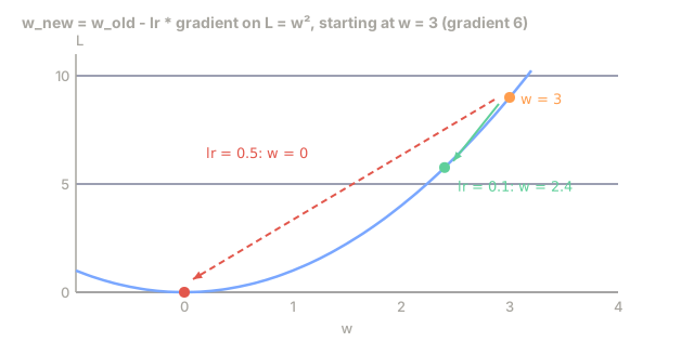
| Learning rate | "How fast it learns" | A scalar that controls the step size when updating weights: w_new = w_old - lr * gradient |
| Topological sort | "The right order" | An ordering of graph nodes where each node appears after all the nodes it depends on, which ensures gradients are fully accumulated before propagation |
| Autograd | "Automatic differentiation" | A system that builds computational graphs during forward computation and automatically computes gradients: what PyTorch's engine does |
Further Reading
- Rumelhart, Hinton & Williams, "Learning representations by back-propagating errors" (1986): the paper that made backpropagation mainstream and unlocked multi-layer network training
- 3Blue1Brown, "Neural Networks" series (https://www.youtube.com/playlist?list=PLZHQObOWTQDNU6R1_67000Dx_ZCJB-3pi): the best visual explanation of backpropagation and gradient flow through networks