Chain Rule & Automatic Differentiation
The chain rule is the entire trick behind training a neural network. Automatic differentiation is just that trick, running as code.
Learning Objectives
- Build a minimal autograd engine (Value class) that records operations and computes gradients via reverse-mode autodiff
- Implement forward and backward passes through a computation graph using topological sort
- Construct and train a multi-layer perceptron on XOR using only the from-scratch autograd engine
- Verify autodiff correctness using gradient checking against numerical finite differences
The Problem
You already know how to take the derivative of a simple function. A neural network is not a simple function. It's hundreds of them, stacked and composed: matrix multiply, add bias, apply an activation, matrix multiply again, softmax, cross-entropy loss. The output is a function of a function of a function, dozens of layers deep.
Training the network means finding the gradient of the loss with respect to every single weight, all at once. By hand, that's impossible for millions of parameters. Numerically, with finite differences, it works, but it's too slow to run at the scale training requires.
The chain rule supplies the math. Automatic differentiation supplies the algorithm. Together, they compute exact gradients through an arbitrary composition of functions, in time proportional to a single forward pass.
This is the actual mechanism behind PyTorch, TensorFlow, and JAX. You're about to build a working miniature of it yourself.
The Concept
The Chain Rule
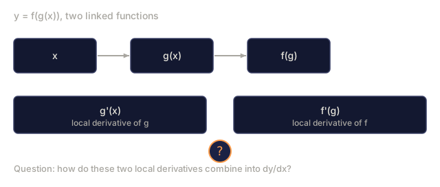
If y = f(g(x)), the derivative of y with respect to x is:
dy/dx = dy/dg * dg/dx = f'(g(x)) * g'(x)
Multiply the derivatives along the chain, one link at a time. Each link contributes its own local derivative.
Take y = sin(x^2) as a concrete example:
g(x) = x^2       g'(x) = 2x
f(g) = sin(g)     f'(g) = cos(g)

dy/dx = cos(x^2) * 2x
Deeper compositions just extend the chain:
y = f(g(h(x)))

dy/dx = f'(g(h(x))) * g'(h(x)) * h'(x)
Every layer in a neural network is one more link.
Computational Graphs
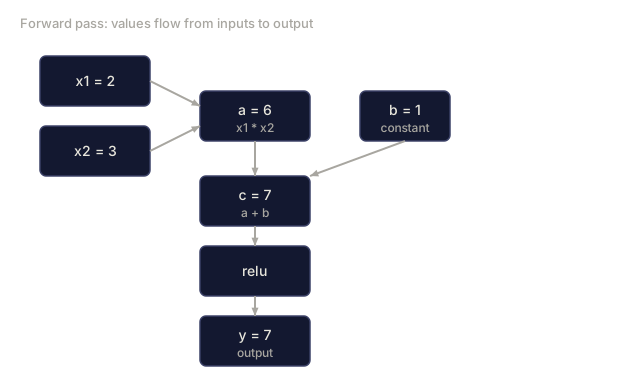
A computational graph makes the chain rule visual. Every operation becomes a node. Data flows forward through the graph. Gradients flow backward through it.
Forward pass (compute values):

Backward pass (compute gradients):

The backward pass applies the chain rule at every node, propagating gradients from the output back to the inputs.
Forward Mode vs Reverse Mode
There are two ways to push the chain rule through a graph.
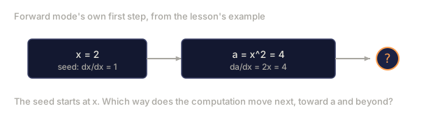
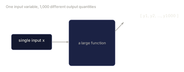
Forward mode starts at the inputs and pushes derivatives forward. It seeds dx/dx = 1 and propagates that through each operation. Good when you have few inputs and many outputs.
Forward mode: seed dx/dx = 1, propagate forward

  x = 2       (dx/dx = 1)
  a = x^2     (da/dx = 2x = 4)
  y = sin(a)  (dy/dx = cos(a) * da/dx = cos(4) * 4 = -2.615)
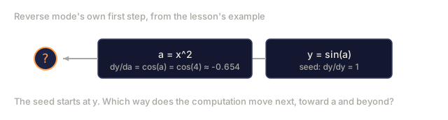
Reverse mode starts at the output and pulls gradients backward. It seeds dy/dy = 1 and propagates that through each operation in reverse. Good when you have many inputs and few outputs.
Reverse mode: seed dy/dy = 1, propagate backward

  y = sin(a)  (dy/dy = 1)
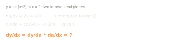
  a = x^2     (dy/da = cos(a) = cos(4) = -0.654)
  x = 2       (dy/dx = dy/da * da/dx = -0.654 * 4 = -2.615)
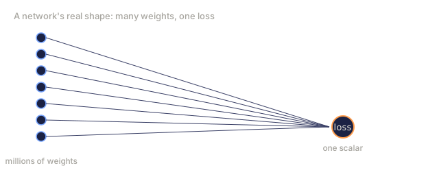
Neural networks have millions of inputs (weights) and exactly one output (loss). Reverse mode computes every gradient in a single backward pass, which is exactly why backpropagation uses reverse mode.
| Mode | Seed | Direction | Best when |
|---|---|---|---|
| Forward | dx_i/dx_i = 1 | Input to output | Few inputs, many outputs |
| Reverse | dy/dy = 1 | Output to input | Many inputs, few outputs (neural nets) |
Dual Numbers for Forward Mode
Forward mode has a clean implementation: dual numbers. A dual number has the form a + b*epsilon, where epsilon^2 = 0.
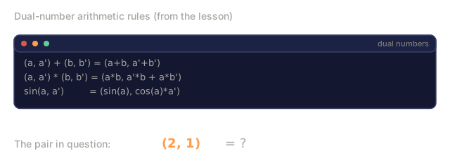
Dual number: (value, derivative)

(2, 1) means: value is 2, derivative w.r.t. x is 1

Arithmetic rules:
  (a, a') + (b, b') = (a+b, a'+b')
  (a, a') * (b, b') = (a*b, a'*b + a*b')
  sin(a, a')         = (sin(a), cos(a)*a')
Seed the input variable with derivative 1, and the derivative propagates automatically through every operation after that.
Building an Autograd Engine
An autograd engine needs three things:
- Value wrapping. Wrap every number in an object that stores its value and its gradient.
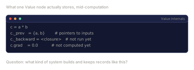
- Graph recording. Every operation records its inputs and the local gradient function used to compute its output.
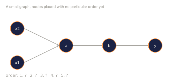
- Backward pass. Topologically sort the graph (order every node so it comes after everything it depends on), then walk it in reverse, applying the chain rule at each node.
This is exactly what PyTorch's autograd does. The torch.Tensor class wraps values, records operations whenever requires_grad=True, and computes gradients the moment you call .backward().
How PyTorch Autograd Works Under the Hood
When you write PyTorch code:
x = torch.tensor(2.0, requires_grad=True)
y = x ** 2 + 3 * x + 1
y.backward()
print(x.grad)  # 7.0 = 2*x + 3 = 2*2 + 3
PyTorch, internally, does five things:
- Creates a
Tensornode forxwithrequires_grad=True. - Every operation (
**,*,+) creates a new node and records the backward function. y.backward()triggers reverse-mode autodiff through the recorded graph.- Each node's
grad_fncomputes local gradients and passes them to parent nodes. - Gradients accumulate in
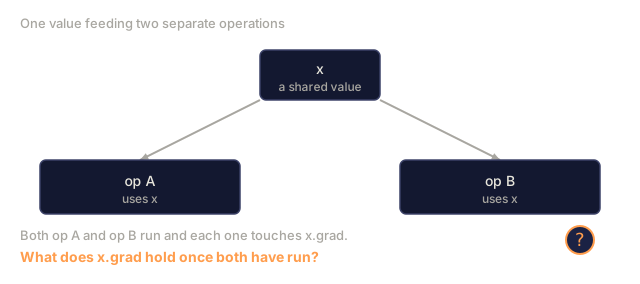
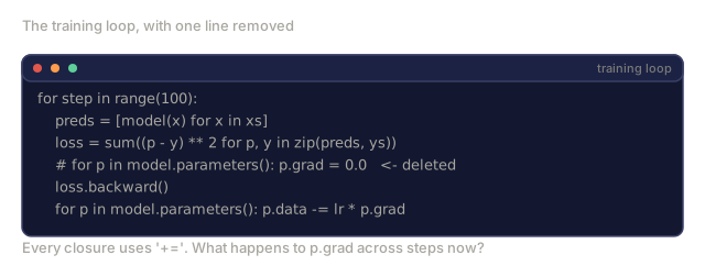
.gradattributes via addition, never replacement.
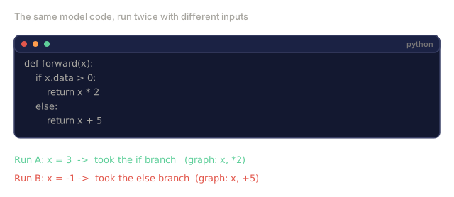
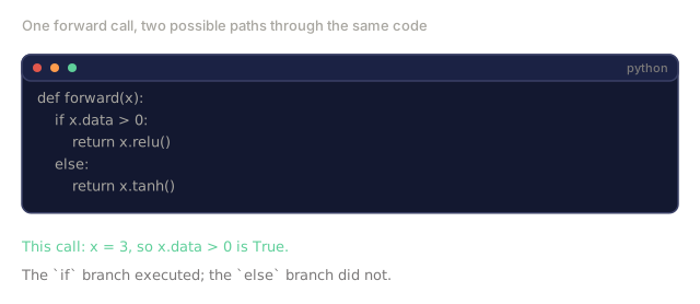
The graph itself is dynamic, built define-by-run: a fresh graph gets constructed on every forward pass. That's exactly why PyTorch supports ordinary Python control flow (if/else, loops) inside a model.

Build It
Step 1: The Value class
class Value:
    def __init__(self, data, children=(), op=''):
        self.data = data
        self.grad = 0.0
        self._backward = lambda: None
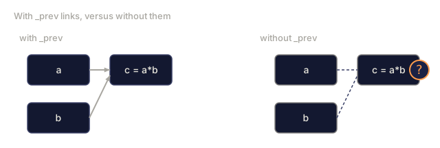
        self._prev = set(children)
        self._op = op

    def __repr__(self):
        return f"Value(data={self.data:.4f}, grad={self.grad:.4f})"
Every Value stores its numeric data, its gradient (initially zero), a backward function, and pointers to child nodes that produced it.
Step 2: Arithmetic operations with gradient tracking
    def __add__(self, other):
        other = other if isinstance(other, Value) else Value(other)
        out = Value(self.data + other.data, (self, other), '+')
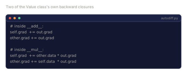
        def _backward():
            self.grad += out.grad
            other.grad += out.grad
        out._backward = _backward
        return out

    def __mul__(self, other):
        other = other if isinstance(other, Value) else Value(other)
        out = Value(self.data * other.data, (self, other), '*')
        def _backward():
            self.grad += other.data * out.grad
            other.grad += self.data * out.grad
        out._backward = _backward
        return out

    def relu(self):
        out = Value(max(0, self.data), (self,), 'relu')
        def _backward():
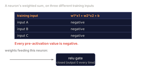
            self.grad += (1.0 if out.data > 0 else 0.0) * out.grad
        out._backward = _backward
        return out
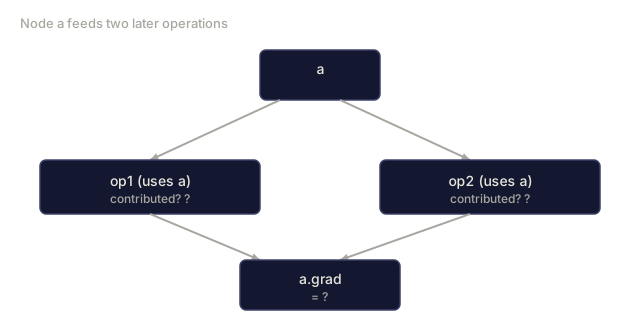
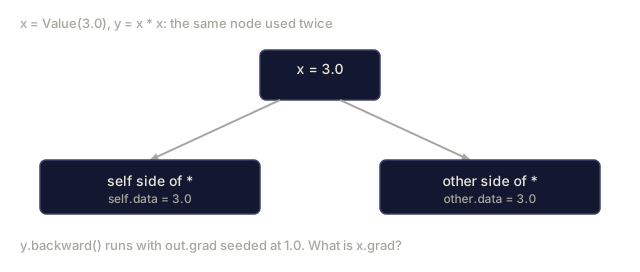
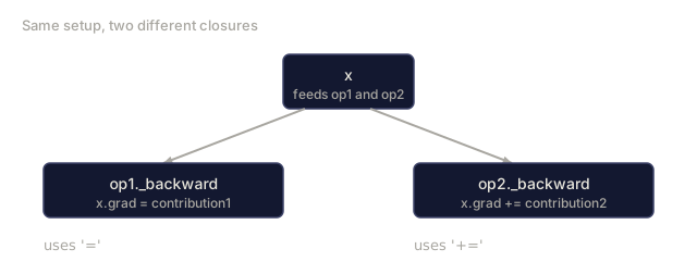
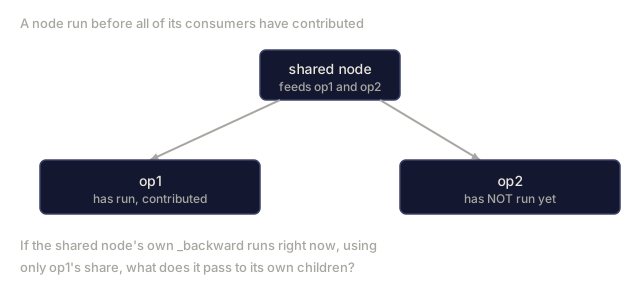
Each operation creates a closure that knows how to compute its own local gradient and multiply that value by the upstream gradient (out.grad). The += matters because a single value can feed into more than one operation, and each one contributes its own share of the gradient.
Step 3: The backward pass
    def backward(self):
        topo = []
        visited = set()
        def build_topo(v):
            if v not in visited:
                visited.add(v)
                for child in v._prev:
                    build_topo(child)
                topo.append(v)
        build_topo(self)

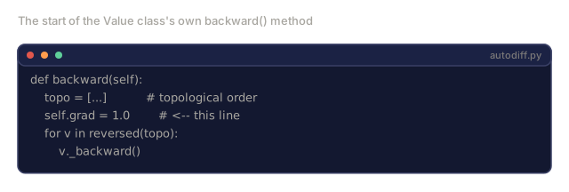
        self.grad = 1.0
        for v in reversed(topo):
            v._backward()
Topologically sorting the graph first ensures every node's gradient is fully computed before it propagates to its children. The seed gradient is 1.0 (dy/dy = 1).
Step 4: More operations for a complete engine
The basic Value class only handles addition, multiplication, and relu. A real autograd engine needs more than that. Here's what you need to actually build neural networks:
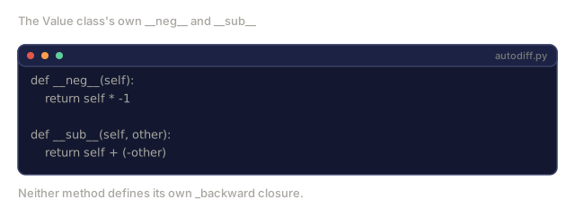
    def __neg__(self):
        return self * -1

    def __sub__(self, other):
        return self + (-other)

    def __radd__(self, other):
        return self + other

    def __rmul__(self, other):
        return self * other

    def __rsub__(self, other):
        return other + (-self)

    def __pow__(self, n):
        out = Value(self.data ** n, (self,), f'**{n}')
        def _backward():
            self.grad += n * (self.data ** (n - 1)) * out.grad
        out._backward = _backward
        return out

    def __truediv__(self, other):
        return self * (other ** -1) if isinstance(other, Value) else self * (Value(other) ** -1)

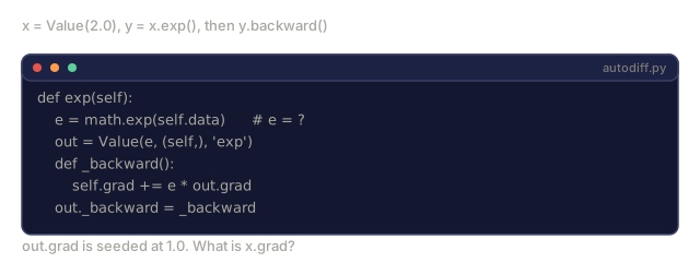
    def exp(self):
        import math
        e = math.exp(self.data)
        out = Value(e, (self,), 'exp')
        def _backward():
            self.grad += e * out.grad
        out._backward = _backward
        return out

    def log(self):
        import math
        out = Value(math.log(self.data), (self,), 'log')
        def _backward():
            self.grad += (1.0 / self.data) * out.grad
        out._backward = _backward
        return out

    def tanh(self):
        import math
        t = math.tanh(self.data)
        out = Value(t, (self,), 'tanh')
        def _backward():
            self.grad += (1 - t ** 2) * out.grad
        out._backward = _backward
        return out
Why each operation matters:
| Operation | Backward rule | Used in |
|---|---|---|
__sub__ | Reuses add + neg | Loss computation (pred - target) |
__pow__ | n * x^(n-1) | Polynomial activations, MSE (error^2) |
__truediv__ | Reuses mul + pow(-1) | Normalization, learning rate scaling |
exp | exp(x) * upstream | Softmax, log-likelihood |
log | (1/x) * upstream | Cross-entropy loss, log probabilities |
tanh | (1 - tanh^2) * upstream | Classic activation function |
The clever part: __sub__ and __truediv__ are defined in terms of existing operations. They get correct gradients for free because the chain rule composes through the underlying add/mul/pow operations.
Step 5: Mini MLP from scratch
With a complete Value class, you can build a neural network. No PyTorch. No NumPy. Just Values and the chain rule.
import random

class Neuron:
    def __init__(self, n_inputs):
        self.w = [Value(random.uniform(-1, 1)) for _ in range(n_inputs)]
        self.b = Value(0.0)

    def __call__(self, x):
        act = sum((wi * xi for wi, xi in zip(self.w, x)), self.b)
        return act.tanh()

    def parameters(self):
        return self.w + [self.b]

class Layer:
    def __init__(self, n_inputs, n_outputs):
        self.neurons = [Neuron(n_inputs) for _ in range(n_outputs)]

    def __call__(self, x):
        return [n(x) for n in self.neurons]

    def parameters(self):
        return [p for n in self.neurons for p in n.parameters()]

class MLP:
    def __init__(self, sizes):
        self.layers = [Layer(sizes[i], sizes[i+1]) for i in range(len(sizes)-1)]

    def __call__(self, x):
        for layer in self.layers:
            x = layer(x)
        return x[0] if len(x) == 1 else x

    def parameters(self):
        return [p for layer in self.layers for p in layer.parameters()]
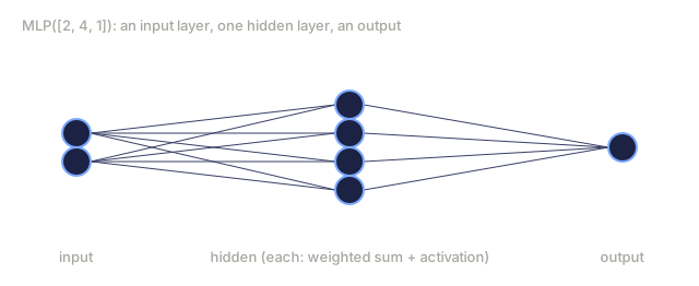
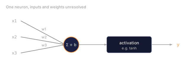
A Neuron computes tanh(w1*x1 + w2*x2 + ... + b). A Layer is a list of neurons. An MLP stacks layers. Every weight is a Value, so calling loss.backward() propagates gradients to every parameter.
Training on XOR:
random.seed(42)
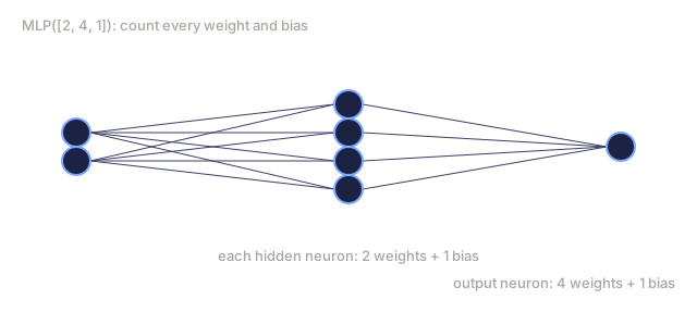
model = MLP([2, 4, 1])  # 2 inputs, 4 hidden neurons, 1 output

xs = [[0, 0], [0, 1], [1, 0], [1, 1]]
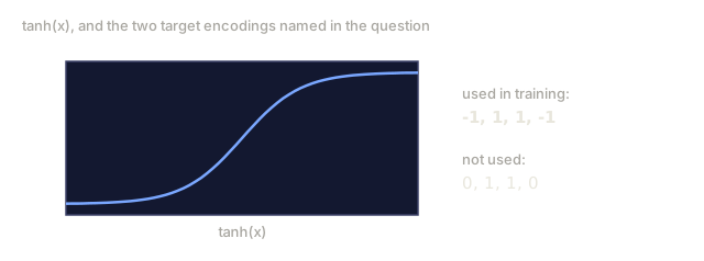
ys = [-1, 1, 1, -1]  # XOR pattern (using -1/1 for tanh)

for step in range(100):
    preds = [model(x) for x in xs]
    loss = sum((p - y) ** 2 for p, y in zip(preds, ys))

    for p in model.parameters():
        p.grad = 0.0
    loss.backward()

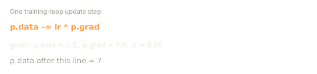
    lr = 0.05
    for p in model.parameters():
        p.data -= lr * p.grad

    if step % 20 == 0:
        print(f"step {step:3d}  loss = {loss.data:.4f}")

print("\nPredictions after training:")
for x, y in zip(xs, ys):
    print(f"  input={x}  target={y:2d}  pred={model(x).data:6.3f}")
This is micrograd. A complete neural network training loop in pure Python with automatic differentiation. Every commercial deep learning framework does the same thing at massive scale.
Step 6: Gradient checking
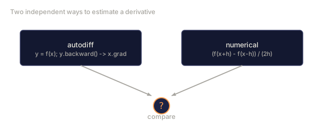
How do you know your autodiff is correct? Compare it against numerical derivatives. This is gradient checking.
def gradient_check(build_expr, x_val, h=1e-7):
    x = Value(x_val)
    y = build_expr(x)
    y.backward()
    autodiff_grad = x.grad

    y_plus = build_expr(Value(x_val + h)).data
    y_minus = build_expr(Value(x_val - h)).data
    numerical_grad = (y_plus - y_minus) / (2 * h)

    diff = abs(autodiff_grad - numerical_grad)
    return autodiff_grad, numerical_grad, diff
Test it on a complex expression:
def expr(x):
    return (x ** 3 + x * 2 + 1).tanh()

ad, num, diff = gradient_check(expr, 0.5)
print(f"Autodiff:  {ad:.8f}")
print(f"Numerical: {num:.8f}")
print(f"Difference: {diff:.2e}")
# Difference should be < 1e-5
Gradient checking is essential when implementing new operations. If your backward pass has a bug, the numerical check catches it. Every serious deep learning implementation runs gradient checks during development.
When to use gradient checking:
| Situation | Do gradient check? |
|---|---|
| Adding a new operation to your autograd | Yes, always |
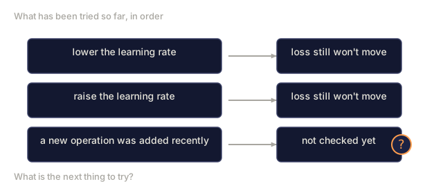
| Debugging a training loop that won't converge | Yes, check gradients first |
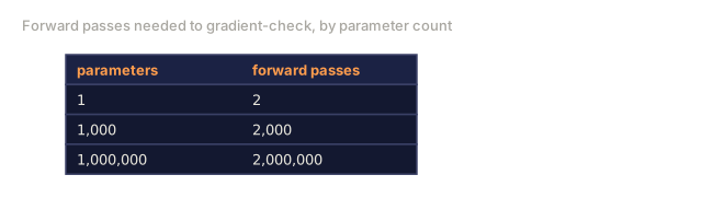
| Production training | No, too slow (2x forward passes per parameter) |
| Unit tests for autograd code | Yes, automate it |
Step 7: Verify against manual calculation
x1 = Value(2.0)
x2 = Value(3.0)
a = x1 * x2          # a = 6.0
b = a + Value(1.0)    # b = 7.0
y = b.relu()          # y = 7.0

y.backward()

print(f"y = {y.data}")          # 7.0
print(f"dy/dx1 = {x1.grad}")   # 3.0 (= x2)
print(f"dy/dx2 = {x2.grad}")   # 2.0 (= x1)
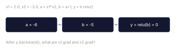
Manual check: y = relu(x1*x2 + 1). Since x1*x2 + 1 = 7 > 0, relu is identity.
dy/dx1 = x2 = 3. dy/dx2 = x1 = 2. The engine matches.
Use It
Verify against PyTorch
import torch

x1 = torch.tensor(2.0, requires_grad=True)
x2 = torch.tensor(3.0, requires_grad=True)
a = x1 * x2
b = a + 1.0
y = torch.relu(b)
y.backward()

print(f"PyTorch dy/dx1 = {x1.grad.item()}")  # 3.0
print(f"PyTorch dy/dx2 = {x2.grad.item()}")  # 2.0
Same gradients. Your engine computes the same result as PyTorch because the math is the same: reverse-mode autodiff via the chain rule.
A more complex expression
a = Value(2.0)
b = Value(-3.0)
c = Value(10.0)
f = (a * b + c).relu()  # relu(2*(-3) + 10) = relu(4) = 4

f.backward()
print(f"df/da = {a.grad}")  # -3.0 (= b)
print(f"df/db = {b.grad}")  #  2.0 (= a)
print(f"df/dc = {c.grad}")  #  1.0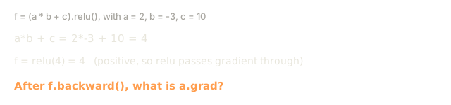
Ship It
This lesson produces:
outputs/skill-autodiff.md: a skill for building and debugging autograd systems.code/autodiff.py: a minimal autograd engine you can keep extending.
The Value class you build here becomes the foundation for the neural network training loop in Phase 3.
The bug that will actually get you here isn't the chain rule, it's the +=. The first time I wrote a Value class, I used = instead of += in a couple of the _backward closures out of habit, the way you would for a variable that's only ever used once. It ran. It printed numbers. Every one of those numbers was wrong, quietly, in a way that only showed up two layers downstream where a shared weight fed two different neurons.
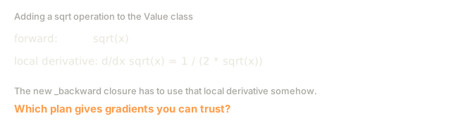
Gradient checking is the only reason I found it in under an hour instead of staring at a loss curve that wouldn't converge and blaming the learning rate. Run the numerical check on every new operation you add to this engine, not just once at the end. It's cheap insurance against a bug that autodiff will never raise an exception for.
Exercises
-
Add
__pow__to the Value class so you can computex ** n. Verify thatd/dx(x^3)atx=2equals12.0. -
Add
tanhas an activation function. Verify thattanh'(0) = 1andtanh'(2) = 0.0707(approx). -
Build a computation graph for a single neuron:
y = relu(w1*x1 + w2*x2 + b). Compute all five gradients and verify against PyTorch. -
Implement forward-mode autodiff using dual numbers. Create a
Dualclass and verify it gives the same derivatives as your reverse-mode engine.
Key Terms
| Term | What people say | What it actually means |
|---|---|---|
| Chain rule | "Multiply the derivatives" | The derivative of composed functions equals the product of each function's local derivative, evaluated at the right point |
| Computational graph | "The network diagram" | A directed acyclic graph where nodes are operations and edges carry values (forward) or gradients (backward) |
| Forward mode | "Push derivatives forward" | Autodiff that propagates derivatives from inputs to outputs. One pass per input variable. |
| Reverse mode | "Backpropagation" | Autodiff that propagates gradients from outputs to inputs. One pass per output variable. |
| Autograd | "Automatic gradients" | A system that records operations on values, builds a graph, and computes exact gradients via the chain rule |
| Dual numbers | "Value plus derivative" | Numbers of the form a + b*epsilon (epsilon^2 = 0) that carry derivative information through arithmetic |
| Topological sort | "Dependency order" | Ordering graph nodes so every node comes after all its dependencies. Required for correct gradient propagation. |
| Gradient accumulation | "Add, don't replace" | When a value feeds into multiple operations, its gradient is the sum of all incoming gradient contributions |
| Dynamic graph | "Define by run" | A computation graph rebuilt on every forward pass, allowing Python control flow inside models (PyTorch style) |
| Gradient checking | "Numerical verification" | Comparing autodiff gradients against numerical finite-difference gradients to verify correctness. Essential for debugging. |
| MLP | "Multi-layer perceptron" | A neural network with one or more hidden layers of neurons. Each neuron computes a weighted sum plus bias, then applies an activation function. |
| Neuron | "Weighted sum + activation" | The basic unit: output = activation(w1x1 + w2x2 + ... + b). The weights and bias are learnable parameters. |
Further Reading
- 3Blue1Brown: Backpropagation calculus — visual explanation of the chain rule in neural networks
- PyTorch Autograd mechanics — how the real system works
- Baydin et al., Automatic Differentiation in Machine Learning: a Survey — comprehensive reference
Code
- autodiff.py (python, 358 lines)
- main.jl (text, 383 lines)