The Perceptron
The perceptron is the atom of neural networks. Split it open: weights, a bias, one decision.
Learning Objectives
- Implement a perceptron from scratch in Python, including the weight update rule and step activation function
- Explain why a single perceptron can only solve linearly separable problems and demonstrate the XOR failure case
- Construct a multi-layer perceptron by composing OR, NAND, and AND gates to solve XOR
- Train a two-layer network with sigmoid activation and backpropagation to learn XOR automatically
The Problem
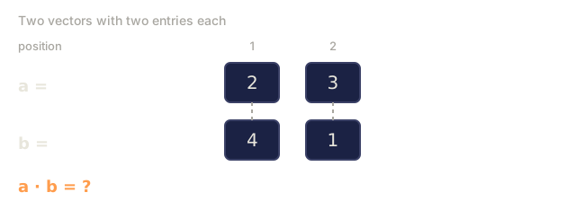
You know vectors and dot products. You know that a matrix transforms inputs into outputs. But how does a machine learn which transformation to use?
The perceptron answers this. It's the simplest possible learning machine: take some inputs, multiply by weights, add a bias, and make a binary decision. Then adjust. That's it. Every neural network ever built is layers of this idea stacked together.
Understanding the perceptron means understanding what "learning" actually means in code: adjusting numbers until the output matches reality.
The Concept
One Neuron, One Decision
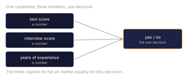
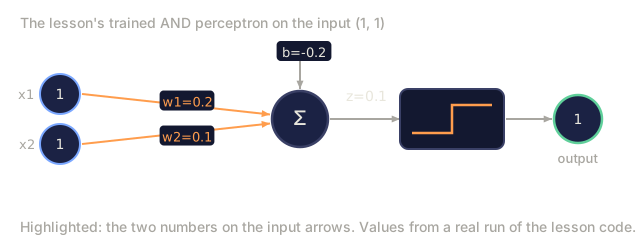
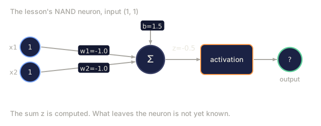
A perceptron takes n inputs, multiplies each by a weight, sums them up, adds a bias, and passes the result through an activation function.
In code, that's a dot product plus a constant:
weighted_sum = sum(w * x for w, x in zip(weights, inputs)) + bias
output = 1 if weighted_sum >= 0 else 0
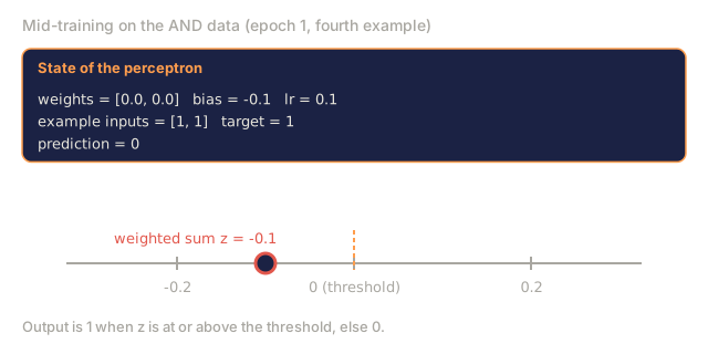
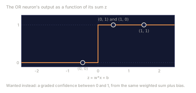
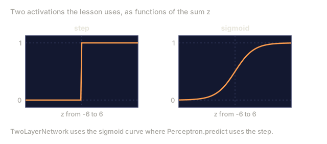
The step function is brutal: if the weighted sum plus bias is >= 0, output 1. Otherwise, output 0.
step(z) = 1  if z >= 0
           0  if z < 0
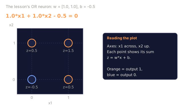
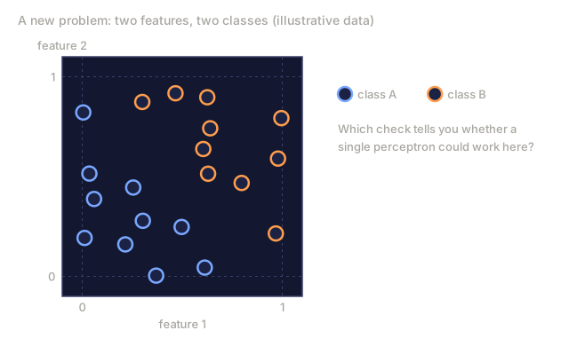
This is a linear classifier. The weights and bias define a line (or hyperplane in higher dimensions) that splits the input space into two regions.
Analogy: think of it as a bouncer working a strict guest list. Your name on the list, how you're dressed, who you showed up with, each counts for a different amount, and the bouncer adds it all up in their head. Clear the threshold (the bias) and you're in. Fall short and you're turned away. No partial credit, no maybe pile, just a yes or a no.
That weighted-sum-plus-bias computation shows up everywhere once you know to look for it:
- Every fully connected layer in a modern network, right before the activation gets applied
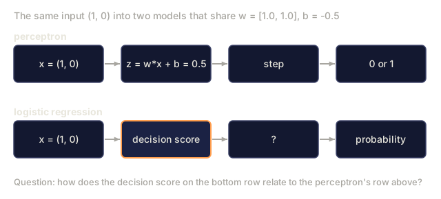
- Logistic regression's decision score: the same perceptron, with sigmoid swapped in for the step function
- A linear SVM's decision function, the sign of w·x + b
- The output neuron of any binary classifier, whatever architecture feeds into it
The Decision Boundary
For two inputs, the perceptron draws a line through 2D space:
  x2
  ┤
  │  Class 1        /
  │    (0)          /
  │                /
  │               / w1·x1 + w2·x2 + b = 0
  │              /
  │             /     Class 2
  │            /        (1)
  ┼───────────/──────────── x1
Everything on one side of the line outputs 0, while everything on the other outputs 1. Training moves this line until it correctly separates the classes.
The Learning Rule
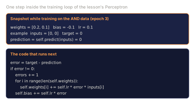
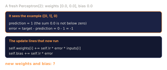
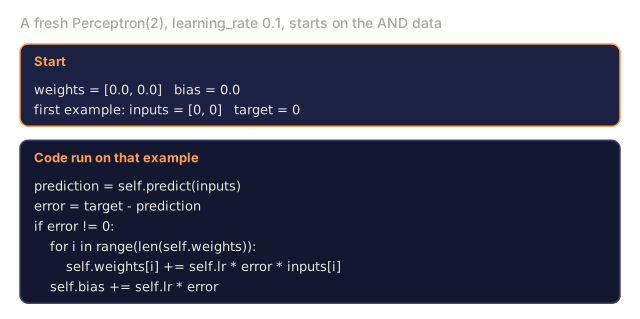
The perceptron learning rule is simple:
For each training example (x, y_true):
    y_pred = predict(x)
    error = y_true - y_pred

    For each weight:
        w_i = w_i + learning_rate * error * x_i
    bias = bias + learning_rate * error
Get the prediction right and error is zero, so nothing moves. Predict 0 when the answer is 1, and the weights climb. Predict 1 when the answer is 0, and they fall. The learning rate sets how big each step is.
Analogy: it's a thermostat that only ever nudges, never jumps. Miss high and it turns the dial down a notch. Miss low and it turns the dial up a notch. Hit the target and it leaves the dial alone. Run that nudge over enough examples and the dial settles wherever the room actually needs it.
The XOR Problem
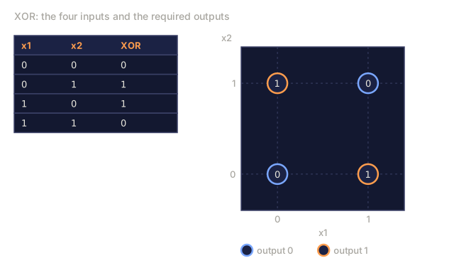
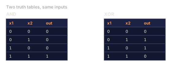
Here's where it breaks. Look at these logic gates:
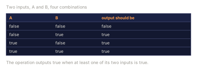
AND gate:           OR gate:            XOR gate:
x1  x2  out         x1  x2  out         x1  x2  out
0   0   0           0   0   0           0   0   0
0   1   0           0   1   1           0   1   1
1   0   0           1   0   1           1   0   1
1   1   1           1   1   1           1   1   0
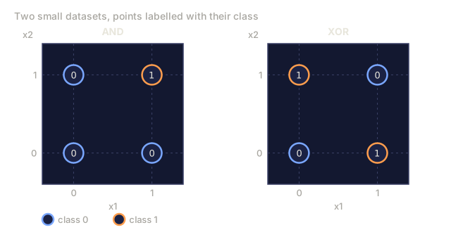
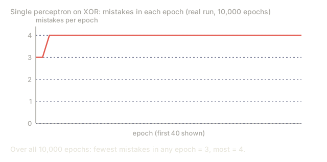
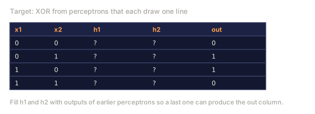
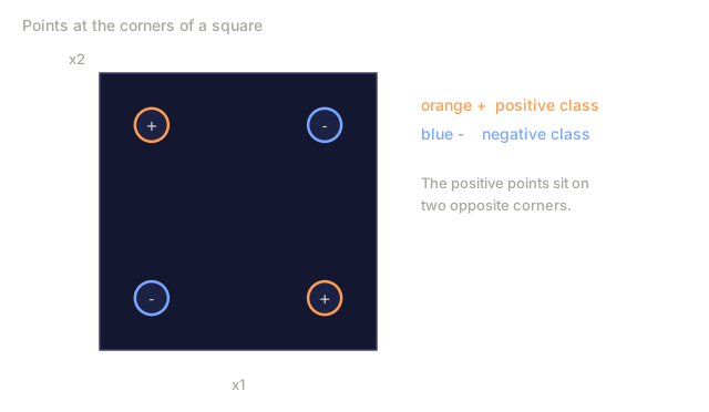
AND and OR are linearly separable: you can draw a single line to separate the 0s from the 1s. XOR is not. No single line can separate [0,1] and [1,0] from [0,0] and [1,1].
AND (separable):        XOR (not separable):

  x2                      x2
  1 ┤  0     1            1 ┤  1     0
    │     /                 │
  0 ┤  0 / 0              0 ┤  0     1
    ┼──/──────── x1         ┼──────────── x1
       line works!          no single line works!
This is a fundamental limit. A single perceptron can only solve linearly separable problems. Minsky and Papert proved this in 1969 and it nearly killed neural network research for a decade.
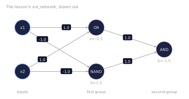
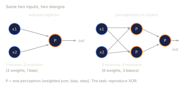
The fix: stack perceptrons into layers. A multi-layer perceptron can solve XOR by combining two linear decisions into a nonlinear one.
Build It
Step 1: The Perceptron class
class Perceptron:
    def __init__(self, n_inputs, learning_rate=0.1):
        self.weights = [0.0] * n_inputs
        self.bias = 0.0
        self.lr = learning_rate

    def predict(self, inputs):
        total = sum(w * x for w, x in zip(self.weights, inputs))
        total += self.bias
        return 1 if total >= 0 else 0

    def train(self, training_data, epochs=100):
        for epoch in range(epochs):
            errors = 0
            for inputs, target in training_data:
                prediction = self.predict(inputs)
                error = target - prediction
                if error != 0:
                    errors += 1
                    for i in range(len(self.weights)):
                        self.weights[i] += self.lr * error * inputs[i]
                    self.bias += self.lr * error
            if errors == 0:
                print(f"Converged at epoch {epoch + 1}")
                return
        print(f"Did not converge after {epochs} epochs")
Step 2: Train on logic gates
and_data = [
    ([0, 0], 0),
    ([0, 1], 0),
    ([1, 0], 0),
    ([1, 1], 1),
]

or_data = [
    ([0, 0], 0),
    ([0, 1], 1),
    ([1, 0], 1),
    ([1, 1], 1),
]

not_data = [
    ([0], 1),
    ([1], 0),
]

print("=== AND Gate ===")
p_and = Perceptron(2)
p_and.train(and_data)
for inputs, _ in and_data:
    print(f"  {inputs} -> {p_and.predict(inputs)}")

print("\n=== OR Gate ===")
p_or = Perceptron(2)
p_or.train(or_data)
for inputs, _ in or_data:
    print(f"  {inputs} -> {p_or.predict(inputs)}")

print("\n=== NOT Gate ===")
p_not = Perceptron(1)
p_not.train(not_data)
for inputs, _ in not_data:
    print(f"  {inputs} -> {p_not.predict(inputs)}")
Step 3: Watch XOR fail
xor_data = [
    ([0, 0], 0),
    ([0, 1], 1),
    ([1, 0], 1),
    ([1, 1], 0),
]

print("\n=== XOR Gate (single perceptron) ===")
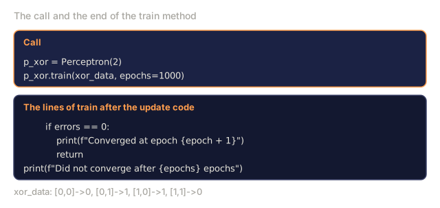
p_xor = Perceptron(2)
p_xor.train(xor_data, epochs=1000)
for inputs, expected in xor_data:
    result = p_xor.predict(inputs)
    status = "OK" if result == expected else "WRONG"
    print(f"  {inputs} -> {result} (expected {expected}) {status}")
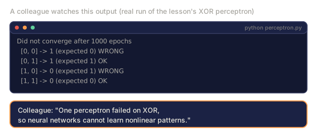
It will never converge. This is the hard proof that a single perceptron cannot learn XOR.
Step 4: Solve XOR with two layers
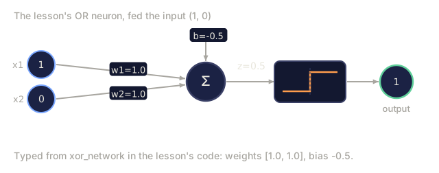
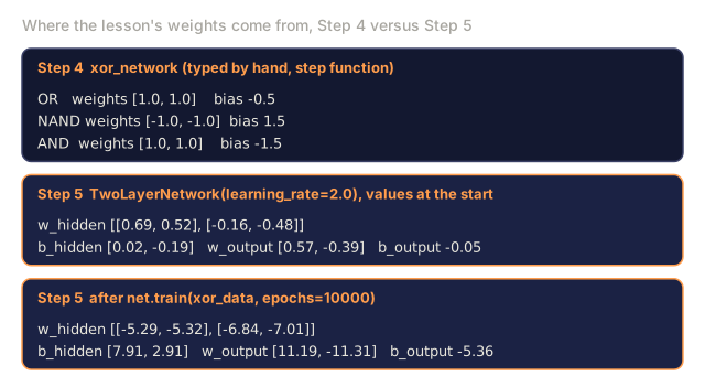
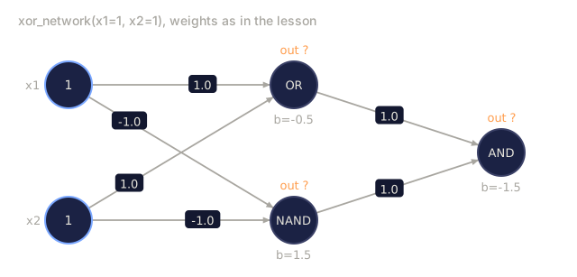
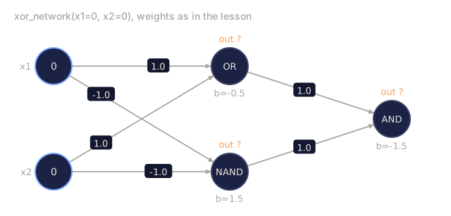
The trick: XOR = (x1 OR x2) AND NOT (x1 AND x2). Combine three perceptrons:

def xor_network(x1, x2):
    or_neuron = Perceptron(2)
    or_neuron.weights = [1.0, 1.0]
    or_neuron.bias = -0.5

    nand_neuron = Perceptron(2)
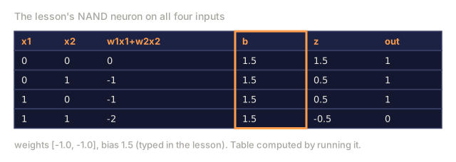
    nand_neuron.weights = [-1.0, -1.0]
    nand_neuron.bias = 1.5

    and_neuron = Perceptron(2)
    and_neuron.weights = [1.0, 1.0]
    and_neuron.bias = -1.5

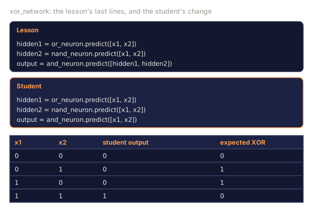
    hidden1 = or_neuron.predict([x1, x2])
    hidden2 = nand_neuron.predict([x1, x2])
    output = and_neuron.predict([hidden1, hidden2])
    return output


print("\n=== XOR Gate (multi-layer network) ===")
for inputs, expected in xor_data:
    result = xor_network(inputs[0], inputs[1])
    print(f"  {inputs} -> {result} (expected {expected})")
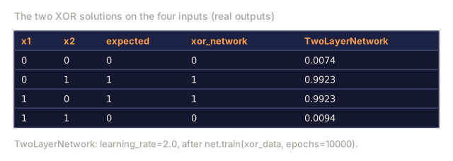
All four cases correct. Stacking perceptrons into layers creates decision boundaries that no single perceptron can produce.
Step 5: Train a Two-Layer Network
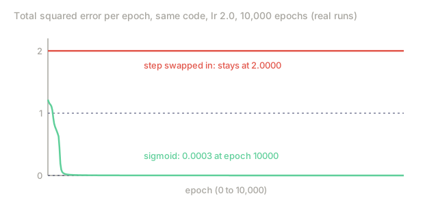
Step 4 hand-wired the weights. That works for XOR, but not for real problems where you don't know the right weights in advance. So swap the activation: replace the step function with sigmoid, and learn the weights automatically through backpropagation.
class TwoLayerNetwork:
    def __init__(self, learning_rate=0.5):
        import random
        random.seed(0)
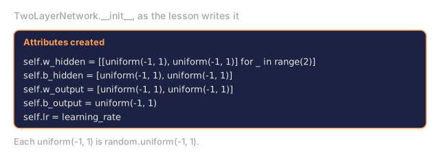
        self.w_hidden = [[random.uniform(-1, 1), random.uniform(-1, 1)] for _ in range(2)]
        self.b_hidden = [random.uniform(-1, 1), random.uniform(-1, 1)]
        self.w_output = [random.uniform(-1, 1), random.uniform(-1, 1)]
        self.b_output = random.uniform(-1, 1)
        self.lr = learning_rate

    def sigmoid(self, x):
        import math
        x = max(-500, min(500, x))
        return 1.0 / (1.0 + math.exp(-x))

    def forward(self, inputs):
        self.inputs = inputs
        self.hidden_outputs = []
        for i in range(2):
            z = sum(w * x for w, x in zip(self.w_hidden[i], inputs)) + self.b_hidden[i]
            self.hidden_outputs.append(self.sigmoid(z))
        z_out = sum(w * h for w, h in zip(self.w_output, self.hidden_outputs)) + self.b_output
        self.output = self.sigmoid(z_out)
        return self.output

    def train(self, training_data, epochs=10000):
        for epoch in range(epochs):
            total_error = 0
            for inputs, target in training_data:
                output = self.forward(inputs)
                error = target - output
                total_error += error ** 2

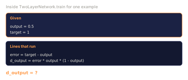
                d_output = error * output * (1 - output)

                saved_w_output = self.w_output[:]
                hidden_deltas = []
                for i in range(2):
                    h = self.hidden_outputs[i]
                    hd = d_output * saved_w_output[i] * h * (1 - h)
                    hidden_deltas.append(hd)

                for i in range(2):
                    self.w_output[i] += self.lr * d_output * self.hidden_outputs[i]
                self.b_output += self.lr * d_output

                for i in range(2):
                    for j in range(len(inputs)):
                        self.w_hidden[i][j] += self.lr * hidden_deltas[i] * inputs[j]
self.b_hidden[i] += self.lr * hidden_deltas[i]net = TwoLayerNetwork(learning_rate=2.0)
net.train(xor_data, epochs=10000)
for inputs, expected in xor_data:
result = net.forward(inputs)
predicted = 1 if result >= 0.5 else 0
print(f" {inputs} -> {result:.4f} (rounded: {predicted}, expected {expected})")Two key differences from Step 4. First, sigmoid replaces the step function: it's smooth, so gradients exist. Second, the train method propagates error backward from output to hidden layer, adjusting every weight proportionally to its contribution to the error. That's backpropagation in 20 lines.
This is the bridge to Lesson 03. The math behind d_output and hidden_deltas is the chain rule applied to the network graph. We'll derive it properly there.
Use It
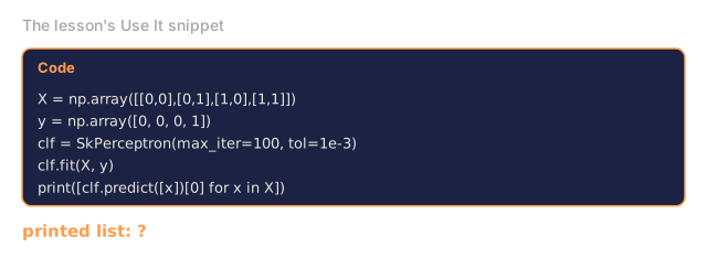
Everything you just built from scratch exists in one import:
from sklearn.linear_model import Perceptron as SkPerceptron
import numpy as np

X = np.array([[0,0],[0,1],[1,0],[1,1]])
y = np.array([0, 0, 0, 1])

clf = SkPerceptron(max_iter=100, tol=1e-3)
clf.fit(X, y)
print([clf.predict([x])[0] for x in X])
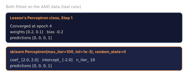
Five lines. Your 30-line Perceptron class does the same thing. The sklearn version adds convergence checks, multiple loss functions, and sparse input support, but the core loop is identical: weighted sum, step function, weight update on error.
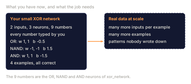
The real gap shows up at scale. What changes in production networks:
- The step function becomes sigmoid, ReLU, or other smooth activations
- Weights are learned automatically via backpropagation (Lesson 03)
- Layers get deeper: 3, 10, 100+ layers
- The same principle holds: each layer creates new features from the previous layer's outputs
A single perceptron can only draw straight lines. Stack them, and you can draw any shape.
Ship It
This lesson produces:
outputs/skill-perceptron.md, a skill covering when to reach for a single-layer perceptron versus a multi-layer network
The XOR failure is worth sitting with longer than most tutorials give it credit for. Minsky and Papert weren't wrong about the math: a single perceptron genuinely cannot solve XOR, full stop. What they got wrong, and what a decade of funding cuts got wrong along with them, was mistaking a limit of one architecture for a limit of the whole idea. Stack two of them and the limit disappears. I think about that every time someone declares a current architecture 'fundamentally incapable' of something. Sometimes that's true. Often it just means nobody found the right way to stack it yet.
The other thing worth doing here, even if you already know backprop cold: type out Step 5 by hand once. Autograd in PyTorch hides d_output and hidden_deltas behind a single call to .backward(). That's the right way to write production code. But skip writing those lines yourself even once, and .backward() stays a black box you trust instead of a shortcut for math you already understand.
Exercises
- Train a perceptron on a NAND gate (the universal gate: any logic circuit can be built from NAND). Verify its weights and bias form a valid decision boundary.
- Modify the Perceptron class to track the decision boundary (w1x1 + w2x2 + b = 0) at each epoch. Print how the line shifts during training on the AND gate.
- Build a 3-input perceptron that outputs 1 only when at least 2 of the 3 inputs are 1 (a majority vote function). Is this linearly separable? Why?
Key Terms
| Term | What people say | What it actually means |
|---|---|---|
| Perceptron | "A fake neuron" | A linear classifier: dot product of inputs and weights, plus bias, through a step function |
| Weight | "How important an input is" | A multiplier that scales each input's contribution to the decision |
| Bias | "The threshold" | A constant that shifts the decision boundary, letting the perceptron fire even with zero inputs |
| Activation function | "The thing that squishes values" | A function applied after the weighted sum: step function for perceptrons, sigmoid/ReLU for modern networks |
| Linearly separable | "You can draw a line between them" | A dataset where a single hyperplane can perfectly separate the classes |
| XOR problem | "The thing perceptrons can't do" | Proof that single-layer networks cannot learn non-linearly-separable functions |
| Decision boundary | "Where the classifier switches" | The hyperplane w*x + b = 0 that divides input space into two classes |
| Multi-layer perceptron | "A real neural network" | Perceptrons stacked in layers, where each layer's output feeds the next layer's input |
Further Reading
- Frank Rosenblatt, "The Perceptron: A Probabilistic Model for Information Storage and Organization in the Brain" (1958) — the original paper that started it all
- Minsky & Papert, "Perceptrons" (1969) — the book that proved XOR was unsolvable by single-layer networks and killed perceptron research for a decade
- Michael Nielsen, "Neural Networks and Deep Learning", Chapter 1 (http://neuralnetworksanddeeplearning.com/) — free online, best visual explanation of how perceptrons compose into networks
Code
- main.jl (text, 232 lines)
- perceptron.py (python, 170 lines)