Support Vector Machines
Find the widest street between two classes. That's the entire idea.
Learning Objectives
- Implement a linear SVM from scratch using hinge loss and gradient descent on the primal formulation
- Explain the maximum margin principle and identify support vectors from a trained model
- Compare linear, polynomial, and RBF kernels and explain how the kernel trick avoids explicit high-dimensional mapping
- Evaluate the tradeoff controlled by the C parameter between margin width and classification errors
The Problem
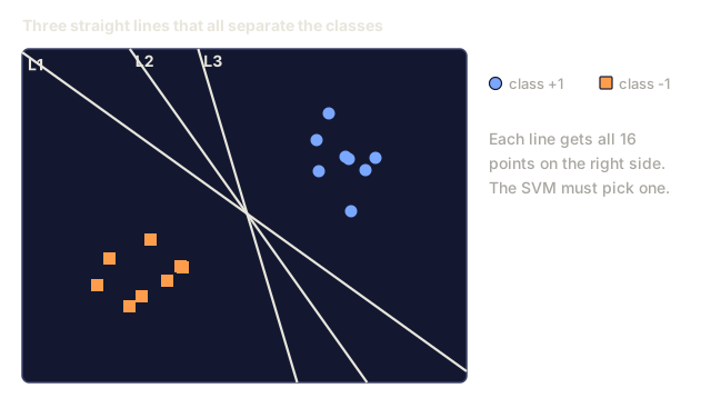
You have two classes of points and need to draw a line, or a hyperplane once you're past two dimensions, that separates them. Infinitely many lines will do the job. Which one should you pick?
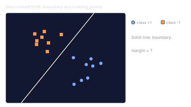
The one with the widest margin. Margin is the distance between the decision boundary and the closest point on either side. Push the boundary as far from both classes as it will go, and you get a classifier that's more confident on the training data and holds up better on points it hasn't seen.
That single idea is the whole Support Vector Machine. Maximize the margin, and the boundary falls out of the math with nothing else bolted on. SVMs ran classification before deep learning took over, and for small datasets, high-dimensional data, or anywhere you want a model with real theoretical guarantees instead of a black box, they still win.
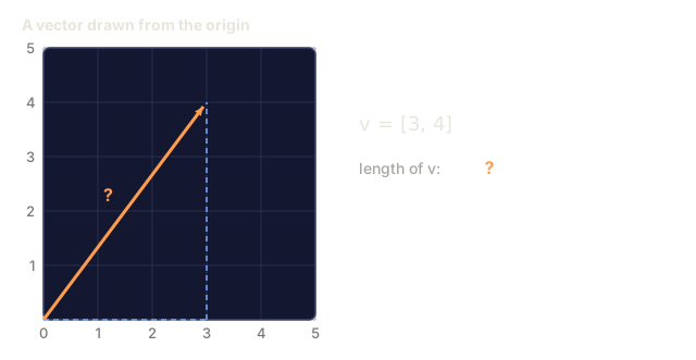
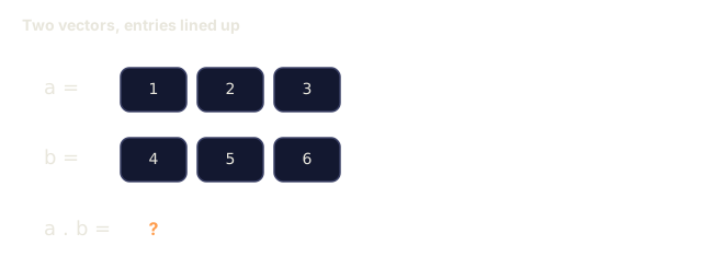
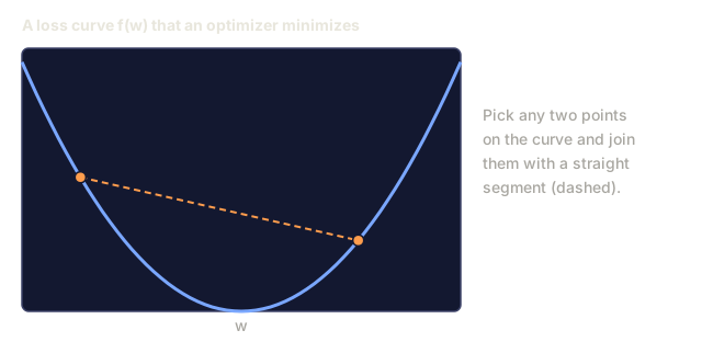
They also lean directly on Phase 1: the optimization is convex (Lesson 18), the margin is measured with norms (Lesson 14), and the kernel trick runs entirely on dot products to handle nonlinear boundaries without ever computing in the high-dimensional space.
The Concept
The maximum margin classifier
Start with linearly separable data: labels y_i in {-1, +1}, feature vectors x_i. We want a hyperplane w^T x + b = 0 that separates the two classes.
The distance from a point x_i to that hyperplane is:
distance = |w^T x_i + b| / ||w||
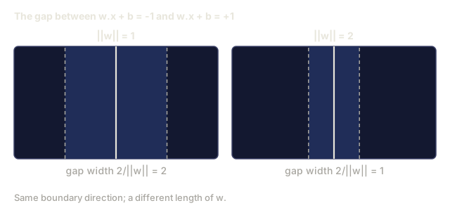
A correctly classified point satisfies y_i * (w^T x_i + b) > 0, and the margin is twice the distance from the hyperplane to the nearest point on either side.

Maximizing the margin gives this optimization problem:
maximize    2 / ||w||     (the margin width)
subject to  y_i * (w^T x_i + b) >= 1  for all i
Flip it to minimizing ||w||^2 instead, and you get the same answer out of friendlier math:
minimize    (1/2) ||w||^2
subject to  y_i * (w^T x_i + b) >= 1  for all i
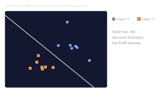
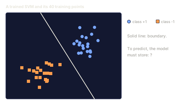
That's a convex quadratic program, so it has one global solution with no local minima hiding anywhere. The points sitting exactly on the margin boundary, where y_i * (w^T x_i + b) = 1, are the support vectors. They're the only points that matter: move or delete any other point and the boundary doesn't move.
Support vectors: the critical few

Most of your training data is dead weight. Only the points touching the margin, the support vectors, decide where the boundary sits. That's also why SVMs are cheap to store at prediction time: keep the support vectors, throw away the rest of the training set.
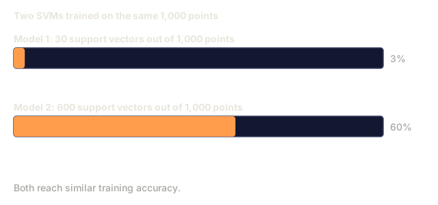
The count of support vectors doubles as a rough bound on generalization error. Fewer support vectors relative to your dataset size means the model is leaning on less of the data to make its call, and it tends to generalize better.
Soft margin: handling noise with the C parameter
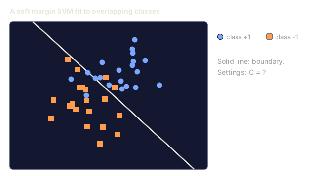
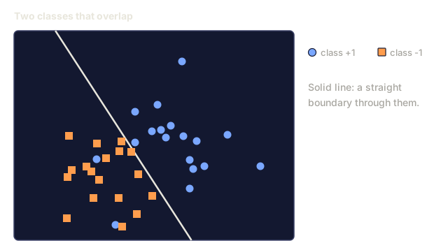
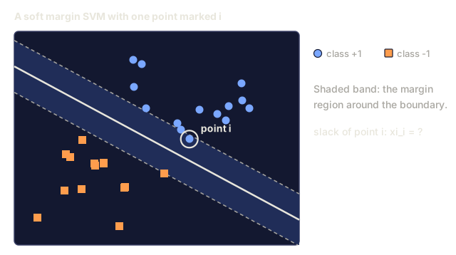
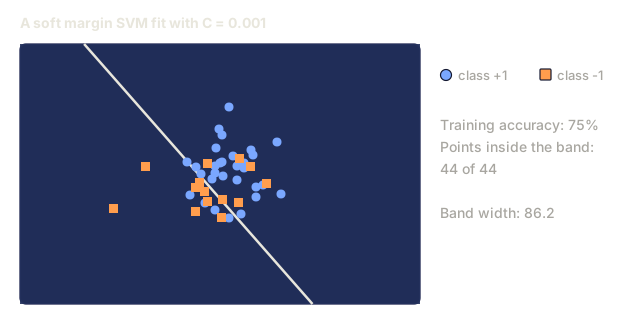
Real data is rarely perfectly separable. Some points end up on the wrong side of the boundary, or inside the margin itself. The soft margin formulation tolerates that by adding slack variables.
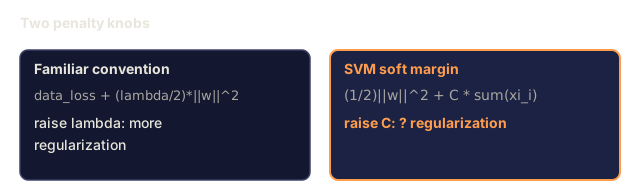
minimize    (1/2) ||w||^2 + C * sum(xi_i)
subject to  y_i * (w^T x_i + b) >= 1 - xi_i
            xi_i >= 0  for all i
Each slack variable xi_i measures how badly point i violates the margin, and C controls how much of that you're willing to tolerate:
| C value | Behavior |
|---|---|
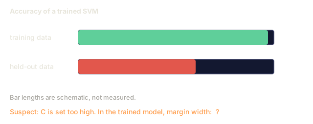
| Large C | Penalizes violations heavily. Narrow margin, fewer misclassifications. Overfits |
| Small C | Allows more violations. Wide margin, more misclassifications. Underfits |
Think of C as regularization strength running backwards: turn it up and you get less regularization, turn it down and you get more.
Hinge loss: the SVM loss function
Drop the constraints and the soft margin SVM turns into an unconstrained optimization:
minimize (1/2) ||w||^2 + C * sum(max(0, 1 - y_i * (w^T x_i + b)))
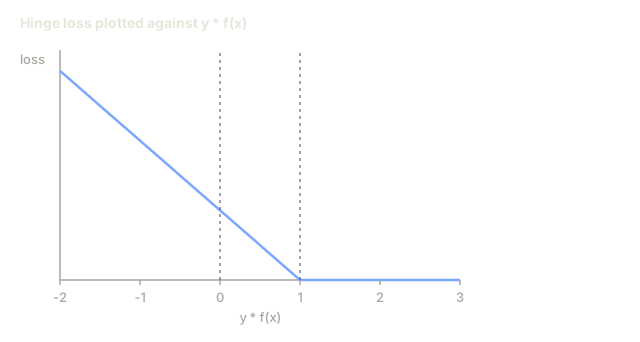
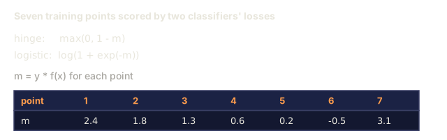
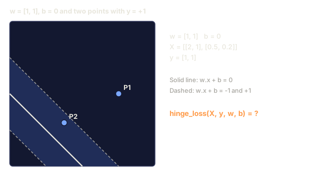
That max(0, 1 - y_i * f(x_i)) term is the hinge loss. It's zero once a point is correctly classified and clear of the margin, and it climbs in a straight line the moment that point drifts inside the margin or gets misclassified.
Hinge loss for a single point:

loss
  |
  | \
  |  \
  |   \
  |    \
  |     \_______________
  |
  +-----|-----|-------->  y * f(x)
       0     1

Zero loss when y*f(x) >= 1 (correctly classified, outside margin).
Linear penalty when y*f(x) < 1.
Line it up against logistic loss, the one behind logistic regression:
Hinge:     max(0, 1 - y*f(x))          Hard cutoff at margin
Logistic:  log(1 + exp(-y*f(x)))        Smooth, never exactly zero
Hinge loss is sparse: only the support vectors contribute anything nonzero to the solution. Logistic loss has no such cutoff, every point pulls its weight, which is exactly why SVMs end up cheaper to store at prediction time.
Training a linear SVM with gradient descent
Skip the constrained QP solver entirely, and you can train a linear SVM with plain gradient descent on hinge loss plus L2 regularization:
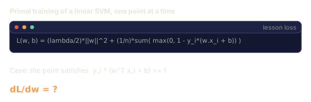
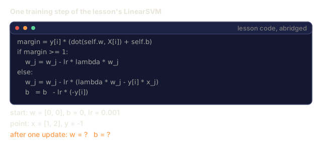
L(w, b) = (lambda/2) * ||w||^2 + (1/n) * sum(max(0, 1 - y_i * (w^T x_i + b)))

Gradient with respect to w:
  If y_i * (w^T x_i + b) >= 1:  dL/dw = lambda * w
  If y_i * (w^T x_i + b) < 1:   dL/dw = lambda * w - y_i * x_i

Gradient with respect to b:
  If y_i * (w^T x_i + b) >= 1:  dL/db = 0
  If y_i * (w^T x_i + b) < 1:   dL/db = -y_i
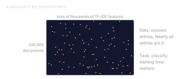
This is the primal formulation, and it runs in O(n * d) per epoch, n samples and d features. On large, sparse, high-dimensional data like text classification, that's fast enough to matter.
The dual formulation and the kernel trick
Take the Lagrangian dual of the SVM problem (Phase 1 Lesson 18 covers the KKT conditions behind it):
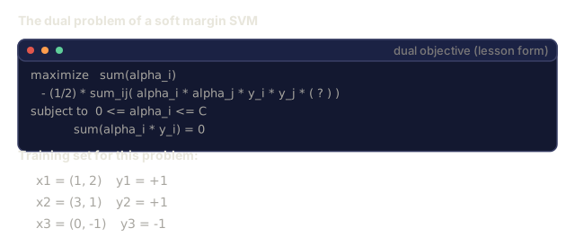
maximize    sum(alpha_i) - (1/2) * sum_ij(alpha_i * alpha_j * y_i * y_j * (x_i . x_j))
subject to  0 <= alpha_i <= C
            sum(alpha_i * y_i) = 0
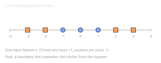
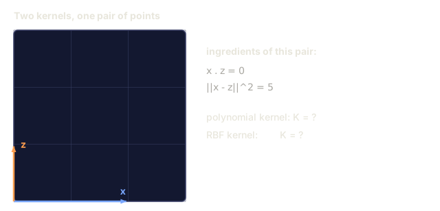
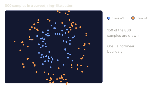
Notice what's actually in there: nothing but dot products x_i . x_j between data points. That's the whole trick. Swap every dot product for a kernel function K(x_i, x_j) and the SVM learns nonlinear boundaries without ever explicitly building the transformed feature space.
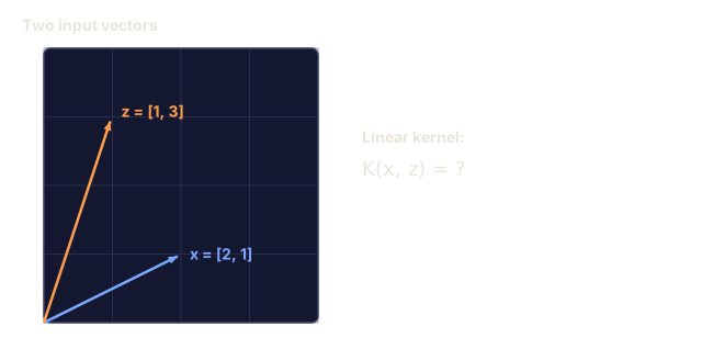
Linear kernel:      K(x, z) = x . z
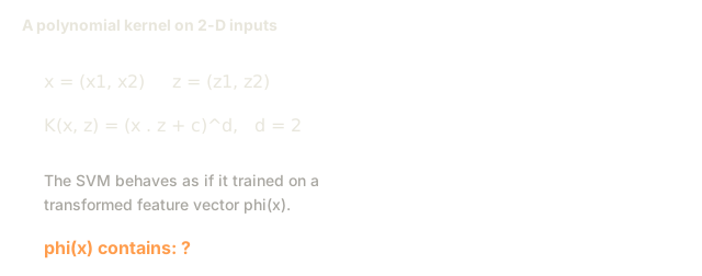
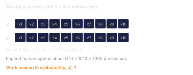
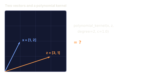
Polynomial kernel:  K(x, z) = (x . z + c)^d
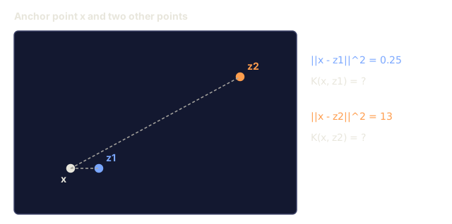
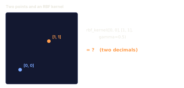
RBF (Gaussian):     K(x, z) = exp(-gamma * ||x - z||^2)
The RBF kernel sends data into an infinite-dimensional space: points close together in the input get a kernel value near 1, points far apart get a value near 0, and the boundary it learns can bend around almost any smooth shape.

What makes this worth caring about: the kernel trick computes a dot product from the high-dimensional space without ever visiting it. A degree-d polynomial kernel in D dimensions implies a feature space with O(D^d) dimensions, yet K(x, z) itself costs only O(D) to compute.
SVM for regression (SVR)
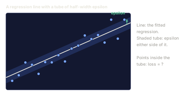
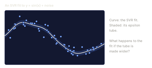
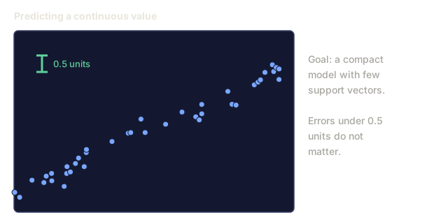
Support Vector Regression takes the same margin idea and fits a tube of width epsilon around the data instead of a boundary between classes. Land inside the tube and it costs nothing; land outside it and the penalty grows linearly with the miss.
minimize    (1/2) ||w||^2 + C * sum(xi_i + xi_i*)
subject to  y_i - (w^T x_i + b) <= epsilon + xi_i
            (w^T x_i + b) - y_i <= epsilon + xi_i*
            xi_i, xi_i* >= 0
Epsilon sets the tube's width, and it's a direct dial on the fit: wider tube, fewer support vectors, smoother curve; narrower tube, more support vectors, tighter fit.
Why SVMs lost to deep learning (and when they still win)
SVMs owned machine learning from the late 1990s through the early 2010s. Deep learning eventually passed them, and the reasons all trace back to scale and raw data:
| Factor | SVMs | Deep learning |
|---|---|---|
| Feature engineering | Requires it | Learns features |
| Scalability | O(n^2) to O(n^3) for kernel | O(n) per epoch with SGD |
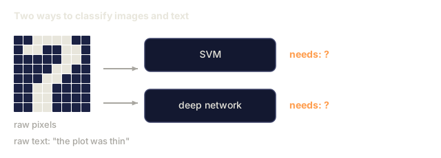
| Image/text/audio | Needs handcrafted features | Learns from raw data |
| Large datasets (>100k) | Slow | Scales well |
| GPU acceleration | Limited benefit | Massive speedup |
But SVMs still win outright in these situations:
- Small datasets (hundreds to low thousands of samples)
- High-dimensional sparse data (text with TF-IDF features)
- When you need mathematical guarantees (margin bounds)
- When training time must be minimal (linear SVM is very fast)
- Binary classification with clear margin structure
- Anomaly detection (one-class SVM)
Build It
Step 1: Hinge loss and gradient
Everything else in this build rests on this one function: hinge loss for a batch, plus its gradient.
def hinge_loss(X, y, w, b):
    n = len(X)
    total_loss = 0.0
    for i in range(n):
        margin = y[i] * (dot(w, X[i]) + b)
        total_loss += max(0.0, 1.0 - margin)
    return total_loss / n
Step 2: Linear SVM via gradient descent
Train by minimizing regularized hinge loss directly. No QP solver, no dual, just gradient descent.
class LinearSVM:
    def __init__(self, lr=0.001, lambda_param=0.01, n_epochs=1000):
        self.lr = lr
        self.lambda_param = lambda_param
        self.n_epochs = n_epochs
        self.w = None
        self.b = 0.0

    def fit(self, X, y):
        n_features = len(X[0])
        self.w = [0.0] * n_features
        self.b = 0.0

        for epoch in range(self.n_epochs):
            for i in range(len(X)):
                margin = y[i] * (dot(self.w, X[i]) + self.b)
                if margin >= 1:
                    self.w = [wj - self.lr * self.lambda_param * wj
                              for wj in self.w]
                else:
                    self.w = [wj - self.lr * (self.lambda_param * wj - y[i] * X[i][j])
                              for j, wj in enumerate(self.w)]
                    self.b -= self.lr * (-y[i])

    def predict(self, X):
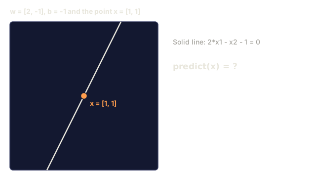
        return [1 if dot(self.w, x) + self.b >= 0 else -1 for x in X]
Step 3: Kernel functions
Linear, polynomial, and RBF, each as a plain function.
def linear_kernel(x, z):
    return dot(x, z)

def polynomial_kernel(x, z, degree=3, c=1.0):
    return (dot(x, z) + c) ** degree

def rbf_kernel(x, z, gamma=0.5):
    diff = [xi - zi for xi, zi in zip(x, z)]
    return math.exp(-gamma * dot(diff, diff))
Step 4: Margin and support vector identification
Once it's trained, pull out which points landed on the margin and measure how wide that margin actually is.
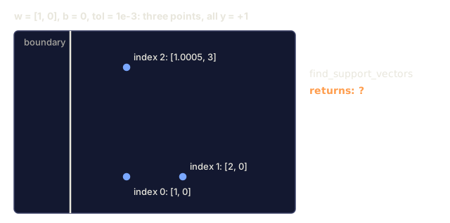
def find_support_vectors(X, y, w, b, tol=1e-3):
    support_vectors = []
    for i in range(len(X)):
        margin = y[i] * (dot(w, X[i]) + b)
        if abs(margin - 1.0) < tol:
            support_vectors.append(i)
    return support_vectors
The full implementation, with every demo, lives in code/svm.py.
Use It
In practice you'll rarely write your own SVM. Here's the scikit-learn version:
from sklearn.svm import SVC, LinearSVC, SVR
from sklearn.preprocessing import StandardScaler
from sklearn.pipeline import Pipeline

clf = Pipeline([
    ("scaler", StandardScaler()),
    ("svm", SVC(kernel="rbf", C=1.0, gamma="scale")),
])
clf.fit(X_train, y_train)
print(f"Accuracy: {clf.score(X_test, y_test):.4f}")
print(f"Support vectors: {clf['svm'].n_support_}")
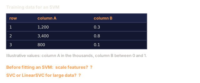
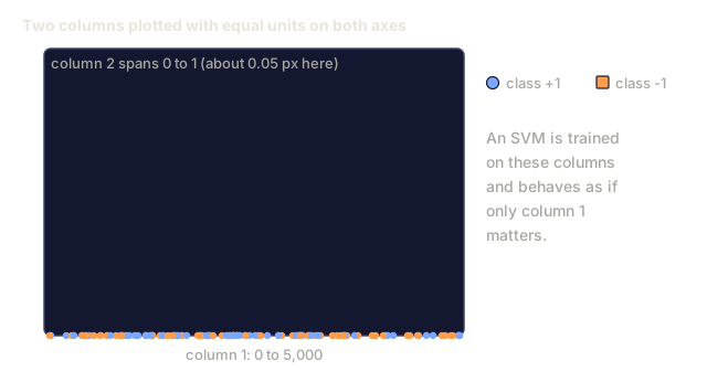
One rule you cannot skip: scale your features first. The margin depends on ||w||, so if one feature ranges into the thousands and another sits between 0 and 1, the geometry is already lying to you before training even starts.
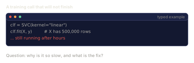
Once your dataset gets large, reach for LinearSVC instead of SVC. LinearSVC runs the primal formulation at O(n) per epoch; SVC's dual formulation costs O(n^2) to O(n^3), which gets painful fast:
from sklearn.svm import LinearSVC

clf = Pipeline([
    ("scaler", StandardScaler()),
    ("svm", LinearSVC(C=1.0, max_iter=10000)),
])
The part of this lesson that actually trips people up in practice isn't the math, it's gamma on the RBF kernel. C gets all the attention because every textbook frames it as the tuning knob, but on real data I've burned more debugging time on a badly chosen gamma than a badly chosen C. Too high, and every training point turns into its own support vector, memorizing noise instead of learning a boundary. Too low, and the model can barely tell the classes apart. Grid search both together. Never tune one and leave the other at its default.
The other thing worth saying out loud: by 2026 you'll reach for an SVM less often than the space it takes up in a curriculum suggests. Gradient boosted trees beat it on almost anything tabular, and neural nets beat it on anything with real structure. Where it still earns its keep is small, clean, high-dimensional datasets, one-class anomaly detection, and any spot where you need a model whose behavior you can actually reason about instead of just trust. Learn it cold anyway. The dual formulation and the kernel trick resurface the moment you start reading papers on kernel methods, Gaussian processes, or kernelized RL, and half the intuition for why the kernel trick even works traces straight back to this lesson.
Exercises
-
Generate a 2D linearly separable dataset. Train your LinearSVM and identify the support vectors. Verify that the support vectors are the points closest to the decision boundary.
-
Vary C from 0.001 to 1000 on a noisy dataset. Plot the decision boundary for each C value. Observe the transition from wide margin (underfitting) to narrow margin (overfitting).
-
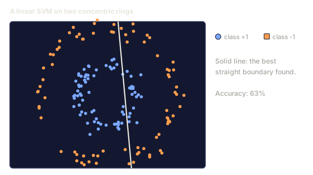
Create a dataset where class boundaries are circular (not linear). Show that a linear SVM fails. Compute the RBF kernel matrix and show that the classes become separable in the kernel-induced feature space.
-
Compare hinge loss vs logistic loss on the same dataset. Train a linear SVM and logistic regression. Count how many training points contribute to each model's decision boundary (support vectors vs all points).
-
Implement SVR (epsilon-insensitive loss). Fit it to y = sin(x) + noise. Plot the epsilon tube around the predictions and highlight the support vectors (points outside the tube).
Key Terms
| Term | What people say | What it actually means |
|---|---|---|
| Support vectors | "The important data points" | The training points closest to the decision boundary. The only points that determine the hyperplane |
| Margin | "How confident the model is" | The distance between the decision boundary and the nearest support vectors. SVMs maximize this |
| Hinge loss | "The SVM's error function" | max(0, 1 - y*f(x)). Zero when correctly classified and outside the margin. Linear penalty otherwise |
| C parameter | "The regularization knob" | Trade-off between margin width and classification errors. Large C = narrow margin, small C = wide margin |
| Soft margin | "Allowing some mistakes" | SVM formulation that allows margin violations via slack variables. Handles non-separable data |
| Kernel trick | "Making the data separable" | Computing dot products in a high-dimensional feature space without explicitly mapping to that space |
| Linear kernel | "No transformation, just similarity" | K(x, z) = x . z. Equivalent to standard dot product. For linearly separable data |
| RBF kernel | "The kernel that works on anything" | K(x, z) = exp(-gamma * ||x-z||^2). Maps to infinite dimensions. Learns any smooth boundary |
| Polynomial kernel | "Curvy decision boundaries" | K(x, z) = (x . z + c)^d. Maps to a feature space of polynomial combinations |
| Dual formulation | "The other way to solve it" | Reformulation of the SVM problem that depends only on dot products between data points. Enables kernels |
| SVR | "SVM, but for regression" | Support Vector Regression. Fits an epsilon-tube around the data. Points inside the tube have zero loss |
| Slack variables | "How far a point crossed the line" | xi_i: measures how much a point violates the margin. Zero for correctly classified points outside margin |
| Maximum margin | "The widest possible gap" | The principle of choosing the hyperplane that maximizes the distance to the nearest points of each class |
Further Reading
- Vapnik: The Nature of Statistical Learning Theory (1995) - the foundational text on SVMs and statistical learning
- Cortes & Vapnik: Support-vector networks (1995) - the original SVM paper
- Platt: Sequential Minimal Optimization (1998) - the SMO algorithm that made SVM training practical
- scikit-learn SVM documentation - practical guide with implementation details
- LIBSVM: A Library for Support Vector Machines - the C++ library behind most SVM implementations