Linear Algebra Intuition
Strip the branding off any AI model and what's left is matrix math.
Learning Objectives
- Implement vector and matrix operations (addition, dot product, matrix multiply) from scratch in Python
- Explain geometrically what the dot product, projection, and Gram-Schmidt process do
- Determine linear independence, rank, and basis of a set of vectors using row reduction
- Connect linear algebra concepts to their AI applications: embeddings, attention scores, and LoRA
The Problem
Open any ML paper and the first page is already covered in vectors, matrices, dot products, and transformations. Without linear algebra intuition, those are just symbols. With it, you can see what a neural network is actually doing — moving points around in space.
You don't need to be a mathematician. You need to see what these operations mean geometrically, then code them yourself.
The Concept
Vectors Are Points (and Directions)
A vector is just a list of numbers. But those numbers mean something: they're coordinates in space.
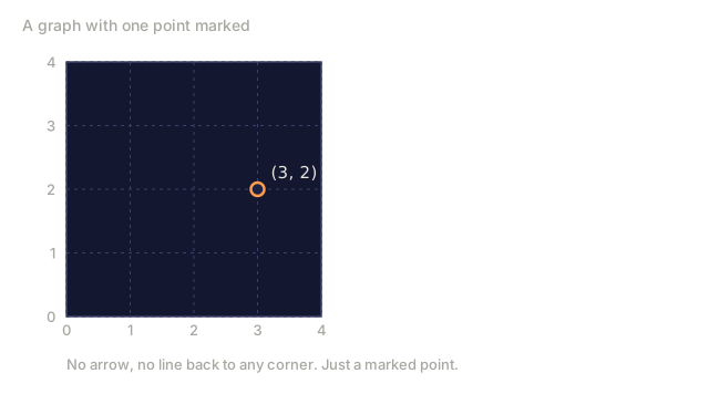
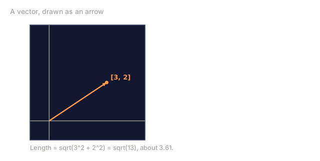
2D vector [3, 2]:
| x | y | Point |
|---|---|---|
| 3 | 2 | The vector points from origin (0,0) to (3, 2) on the plane |
The vector has magnitude sqrt(3^2 + 2^2) = sqrt(13) and points up and to the right.

In code, that list of numbers is exactly what gets stored. There's no special "vector" type the language needs:
v = [3, 2]             # plain Python list
v = np.array([3, 2])   # NumPy array -- what you'll actually use
The vector is the array. Every operation covered below (add, dot product, magnitude) is just an operation on that array's elements, whether you write the loop yourself (Build It) or call NumPy (Use It).
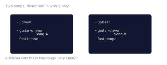
Analogy: think of a vector as a taste profile, like the numbers behind a music app's recommendations: how much you like rock, how much jazz, how much hip-hop. Two people with similar profiles probably enjoy the same songs. A word embedding works the same way, just with hundreds of made-up "taste" dimensions instead of three genres.
In AI, vectors represent everything:
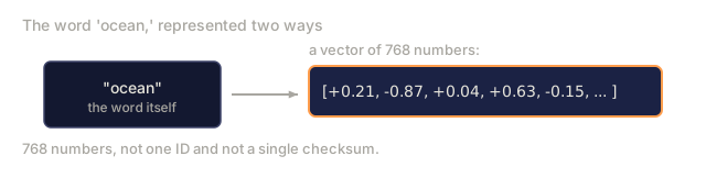
- A word → a vector of 768 numbers (its "meaning" in embedding space)
- An image → a vector of millions of pixel values
- A user → a vector of preferences
Matrices Are Transformations
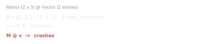
A matrix is a grid of numbers arranged in rows and columns. A matrix with m rows and n columns is called "m by n":
2x3 matrix:
| col 1 | col 2 | col 3 | |
|---|---|---|---|
| row 1 | 1 | 0 | 2 |
| row 2 | -1 | 3 | 1 |
This one has 2 rows and 3 columns, so it's a 2x3 matrix.
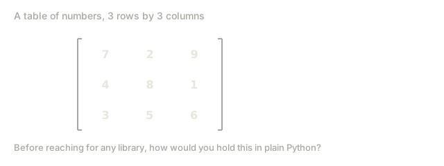
In code, a matrix is just a list of rows, or more commonly a 2D NumPy array:
M = [[1, 0, 2], [-1, 3, 1]]            # plain Python: a list of rows
M = np.array([[1, 0, 2], [-1, 3, 1]])  # NumPy -- what you'll actually use
Each inner list becomes one row, and M.shape reports (2, 3).
A matrix is more than a static grid, though. It also transforms one vector into another: it can rotate, scale, stretch, or project.


Every operation below (matrix multiply, transpose) is just indexing into that array's rows and columns, whether you write the loops yourself (Build It) or call NumPy (Use It).
Analogy: picture a mixing board in a recording studio. Each knob blends some of the input channels into an output channel, and turning every knob at once transforms the whole sound. A neural network layer works the same way: a matrix of "knobs" that blends an input vector into a new output vector.
In AI, matrices ARE the model:
- Neural network weights → matrices that transform input into output
- Attention scores → matrices that decide what to focus on
- Embeddings → matrices that map words to vectors
The Dot Product Measures Similarity
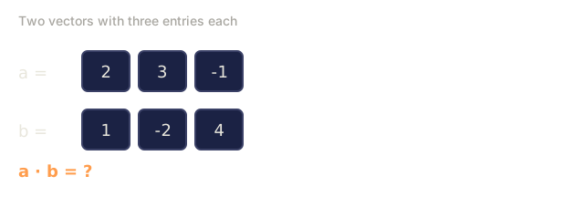
The dot product of two vectors is a single number: multiply each pair of matching components, then add up the results.
a · b = a₁×b₁ + a₂×b₂ + ... + aₙ×bₙ
Example: a = [1, 2, 3], b = [4, 5, 6]
a · b = 1×4 + 2×5 + 3×6 = 4 + 10 + 18 = 32
In code:
a = [1, 2, 3]
b = [4, 5, 6]
dot = sum(x * y for x, y in zip(a, b))   # 32

import numpy as np
dot = np.dot(a, b)   # 32 -- what you'll actually use
That single number turns out to tell you how similar two vectors are:
Same direction:      a · b > 0  (similar)
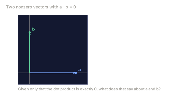
Perpendicular:       a · b = 0  (unrelated)
Opposite direction:  a · b < 0  (dissimilar)

Analogy: it's like comparing two shopping carts item by item. Multiply the quantity of each matching item and add it up: two carts full of the same items in similar amounts score high (similar), carts with nothing in common score zero, and a cart that's the exact opposite of another scores negative. A recommendation engine matches your "cart" of interests against every product's the same way.
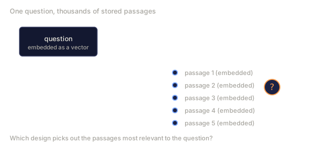
This is literally how search engines, recommendation systems, and RAG (retrieval-augmented generation, where the model looks up relevant text before answering) work — find vectors with high dot products.
Linear Independence
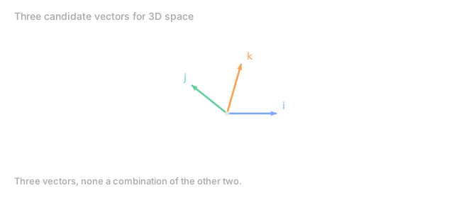
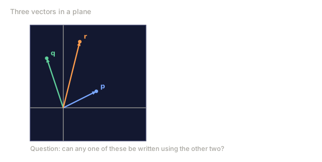
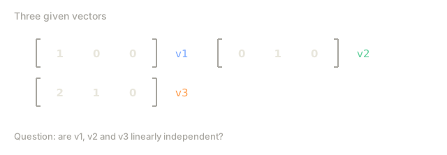
Vectors are linearly independent if no vector in the set can be written as a combination of the others. If v1, v2, v3 are independent, they span a 3D space. If one is a combination of the others, they only span a plane.
Concrete example:
v1 = [1, 0, 0]
v2 = [0, 1, 0]
v3 = [2, 1, 0]   # v3 = 2*v1 + v2
v1 and v2 are independent: neither is a scalar multiple or combination of the other. But v3 = 2*v1 + v2, so {v1, v2, v3} is a dependent set. All three vectors lie in the xy-plane, and no combination of them reaches [0, 0, 1]. Three vectors, but only two dimensions of freedom.

In code, you can check this with the matrix rank: if the rank is less than the number of vectors, the set is dependent.
import numpy as np

vectors = np.array([[1, 0, 0], [0, 1, 0], [2, 1, 0]])
rank = np.linalg.matrix_rank(vectors)
print(rank < len(vectors))   # True -- the set is linearly dependent
Analogy: imagine paying two weather forecasters who always give the identical forecast. The second one is linearly dependent on the first: no matter how you combine their reports, you still only know one thing, rain or not, not two independent opinions. A model with duplicate features is paying for the same forecast twice.
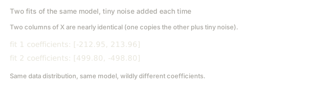
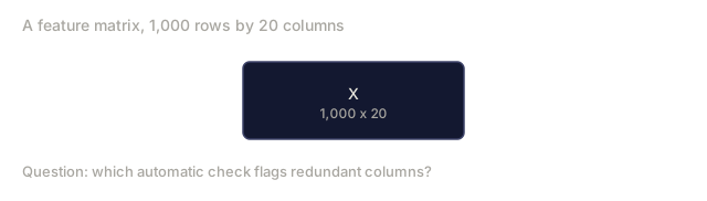
Why it matters for AI: your feature matrix should have linearly independent columns. If two features are perfectly correlated (linearly dependent), the model cannot distinguish their effects. This causes multicollinearity in regression: the weight matrix becomes unstable, and small input changes produce wild output swings.
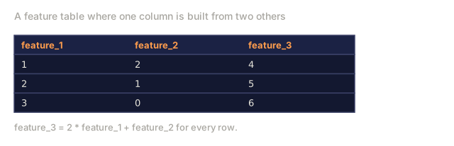
In a dataset: if feature_3 = 2*feature_1 + feature_2, adding feature_3 gives the model zero new information. Worse, it makes the normal equations (the system of equations you solve to fit a linear regression) singular, so there is no unique solution for the weights.
Basis and Rank
A basis is a minimal set of linearly independent vectors that span the entire space. The number of basis vectors is the dimension of the space.
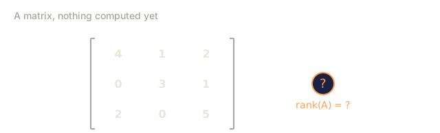
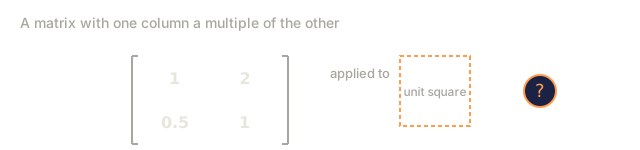
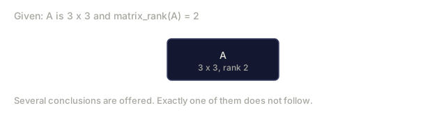
Rank of a matrix is the number of linearly independent columns it has, which equals the number of linearly independent rows.
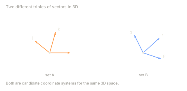
The standard basis for 3D space is {[1,0,0], [0,1,0], [0,0,1]}. But any three independent vectors in 3D form a valid basis. The choice of basis is a choice of coordinate system.
In code, a basis is just a matrix whose rows are those vectors, and you confirm it's valid by checking that its rank equals the number of vectors:
import numpy as np

standard_basis = np.array([[1, 0, 0], [0, 1, 0], [0, 0, 1]])
print(np.linalg.matrix_rank(standard_basis) == 3)   # True -- a valid basis for 3D
Analogy: think of a basis like the smallest set of primary paint colors, red, yellow, and blue, needed to mix any color you want. Rank is how many genuinely different colors are actually in your paint set: hand someone a "purple" that's secretly just red and blue already mixed, and it doesn't add a new color. Your rank stays at 2 no matter how many tubes are on the table.
In code:
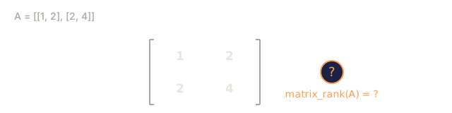
A = np.array([[1, 2], [2, 4]])
print(np.linalg.matrix_rank(A))   # 1 -- the second column is just 2x the first
If rank < min(rows, cols), the matrix is rank-deficient. This means:
- The system has infinitely many solutions (or none)
- Information is lost in the transformation
- The matrix cannot be inverted

| Situation | Rank | What it means for ML |
|---|---|---|
| Full rank (rank = min(m, n)) | Maximum possible | Unique least-squares solution exists. Model is well-conditioned. |
| Rank deficient (rank < min(m, n)) | Below maximum | Features are redundant. Infinitely many weight solutions. Needs regularization (a penalty added to the loss that forces one well-behaved solution). |
| Rank 1 | 1 | Every column is a scaled copy of one vector. All data lies on a line. |
| Near rank-deficient (small singular values) | Numerically low | Matrix is ill-conditioned. Tiny input noise causes large output changes. Fix it with SVD truncation or ridge regression (both covered in later lessons in this phase). |
Projection
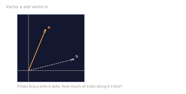
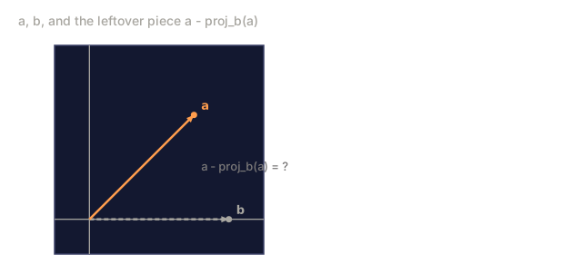
Projecting vector a onto vector b gives the component of a in the direction of b:
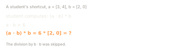
proj_b(a) = (a dot b / b dot b) * b
Example: a = [3, 4], b = [1, 0]
proj_b(a) = (31 + 40) / (11 + 00) * [1, 0] = 3 * [1, 0] = [3, 0]
In code:
import numpy as np

a = np.array([3, 4])
b = np.array([1, 0])
proj = (np.dot(a, b) / np.dot(b, b)) * b
print(proj)   # [3, 0]

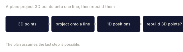
The residual (a - proj_b(a)) is perpendicular to b. This orthogonal decomposition is the foundation of least-squares fitting: choosing the line or plane that makes the total squared error between it and the data as small as possible. The projection drops the y-component here, which is dimensionality reduction in its simplest form: throw away the directions you don't care about.
Analogy: it's like a shadow. Shine a light straight down on vector a onto the line through b, and the shadow it casts is proj_b(a). PCA does this to an entire dataset at once: it finds the single best wall to shine the light on so the shadows keep as much of the data's original spread as possible.
Projection is everywhere in ML:
- Linear regression minimizes the distance from observations to the column space — the solution IS a projection
- PCA projects data onto the directions of maximum variance
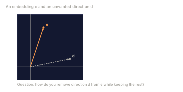
- Removing an unwanted direction from a representation (bias/concept ablation in embeddings) works by projecting it out: subtract the component along that direction and keep the rest
Gram-Schmidt Process
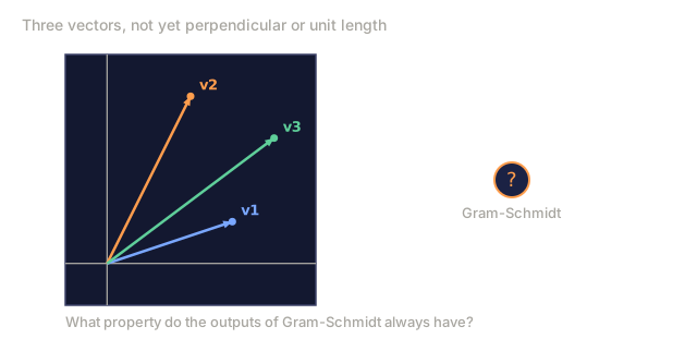
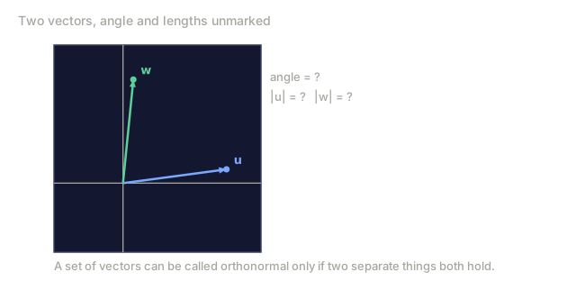
Gram-Schmidt converts any set of independent vectors into an orthonormal basis. Orthonormal means every vector has length 1 and every pair is perpendicular.
The algorithm:
- Take the first vector, normalize it
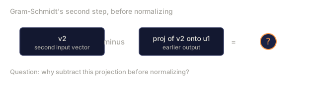
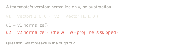
- Take the second vector, subtract its projection onto the first, normalize
- Take the third vector, subtract its projections onto all previous vectors, normalize
- Repeat for remaining vectors
Input:  v1, v2, v3, ... (linearly independent)

u1 = v1 / |v1|

w2 = v2 - (v2 dot u1) * u1
u2 = w2 / |w2|

w3 = v3 - (v3 dot u1) * u1 - (v3 dot u2) * u2
u3 = w3 / |w3|

Output: u1, u2, u3, ... (orthonormal basis)
Analogy: it's like tidying a messy bookshelf into non-overlapping categories. Take each new book, strip out whatever already belongs to a category you've filed, and shelve the pure leftover as its own new category. Do that for every book and you end up with categories that share nothing in common with each other, which is exactly what "orthogonal" means here.
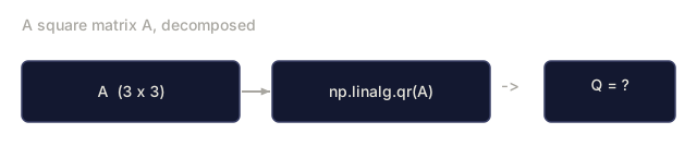
This is how QR decomposition works internally. Q is the orthonormal basis, R captures the projection coefficients. QR decomposition is used in:
- Solving linear systems (more stable than Gaussian elimination)
- Computing eigenvalues (QR algorithm)
- Least-squares regression (the standard numerical method)
Eigenvectors and Eigenvalues
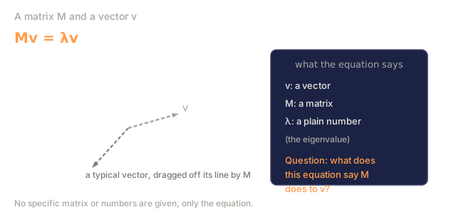
An eigenvector of a matrix is a vector that keeps pointing along the same line after the matrix transforms it: it only gets longer or shorter, never rotated, and the factor it stretches by is the eigenvalue. Most vectors don't get this treatment — a matrix drags them off at an angle, away from the line they started on.
Mv = λv
Here v is the eigenvector and λ (a plain number, not a vector) is the eigenvalue. Every other vector maps somewhere off that line; only along v does the output stay parallel to the input.
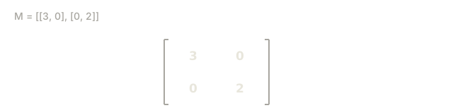
Simplest case: M = [[3, 0], [0, 2]]. This stretches the x-axis by 3 and the y-axis by 2, and drags every other direction toward whichever axis stretches more. The x- and y-axes are the eigenvectors here, with eigenvalues 3 and 2.
Add an off-diagonal term and the eigenvectors rotate away from the x/y axes, but for a symmetric matrix (the same value in both off-diagonal spots) they stay perpendicular to each other. In code:
import numpy as np

M = np.array([[2.0, 0.8], [0.8, 1.0]])
eigenvalues, eigenvectors = np.linalg.eig(M)
print(eigenvalues)    # how much each axis stretches
print(eigenvectors)   # the two axes, as columns
The widget below makes that matrix draggable. a and d set how much the matrix stretches along the x- and y-directions, and off-diagonal b adds the shear that rotates the eigenvectors away from those axes. The dashed lines are the eigenvectors: fixed directions that never rotate no matter what the sliders are set to, only stretch. The orange arrows are those same axes, scaled by their eigenvalues. The grey arrow is a plain input vector at whatever angle you set; the blue arrow is where the matrix sends it. Off the dashed axes, the blue arrow both stretches and swings toward a new direction. Drag the angle slider around the full circle and watch: only when the grey arrow crosses a dashed line does the blue arrow stay pointing exactly the same way.
Analogy: picture kneading dough on a counter. Push straight down and it spreads out in every direction, but along a couple of specific directions the dough was already flowing that way, so pressing there just stretches it further without twisting it sideways. Every other direction gets dragged off at an angle by the push.
PCA finds its axes by computing the eigenvectors of a covariance matrix. Spectral clustering, PageRank, and the stability of gradient descent near a minimum all come down to the same question this widget is asking: which directions does a matrix merely scale, and by how much? Matrix Transformations and Singular Value Decomposition, later in this phase, cover the full computation; this is just the geometry to carry forward.
Build It
Step 1: Vectors from scratch (Python)
class Vector:
    def __init__(self, components):
        self.components = list(components)
        self.dim = len(self.components)

    def __add__(self, other):
        return Vector([a + b for a, b in zip(self.components, other.components)])

    def __sub__(self, other):
        return Vector([a - b for a, b in zip(self.components, other.components)])

    def dot(self, other):
        return sum(a * b for a, b in zip(self.components, other.components))

    def magnitude(self):
        return sum(x**2 for x in self.components) ** 0.5

    def normalize(self):
        mag = self.magnitude()
        return Vector([x / mag for x in self.components])

    def cosine_similarity(self, other):
        return self.dot(other) / (self.magnitude() * other.magnitude())

    def __repr__(self):
        return f"Vector({self.components})"


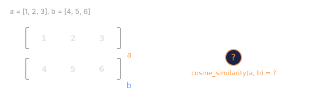
a = Vector([1, 2, 3])
b = Vector([4, 5, 6])

print(f"a + b = {a + b}")
print(f"a · b = {a.dot(b)}")
print(f"|a| = {a.magnitude():.4f}")
print(f"cosine similarity = {a.cosine_similarity(b):.4f}")
Step 2: Matrices from scratch (Python)
class Matrix:
    def __init__(self, rows):
        self.rows = [list(row) for row in rows]
        self.shape = (len(self.rows), len(self.rows[0]))

    def __matmul__(self, other):
        if isinstance(other, Vector):
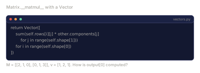
            return Vector([
                sum(self.rows[i][j] * other.components[j] for j in range(self.shape[1]))
                for i in range(self.shape[0])
            ])
        rows = []
        for i in range(self.shape[0]):
            row = []
            for j in range(other.shape[1]):
                row.append(sum(
                    self.rows[i][k] * other.rows[k][j]
                    for k in range(self.shape[1])
                ))
            rows.append(row)
        return Matrix(rows)

    def transpose(self):
        return Matrix([
            [self.rows[j][i] for j in range(self.shape[0])]
            for i in range(self.shape[1])
        ])

    def __repr__(self):
        return f"Matrix({self.rows})"


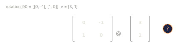
rotation_90 = Matrix([[0, -1], [1, 0]])
point = Vector([3, 1])

rotated = rotation_90 @ point
print(f"Original: {point}")
print(f"Rotated 90°: {rotated}")
Step 3: Why this matters for AI
import random

random.seed(42)
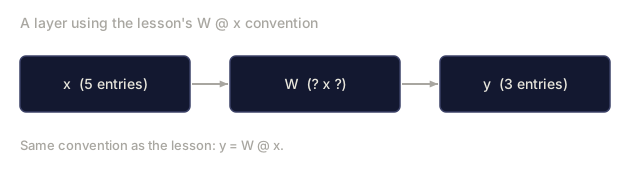
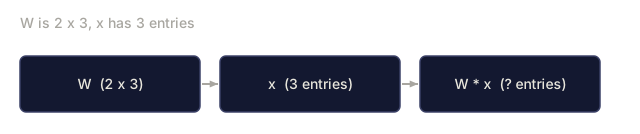
weights = Matrix([[random.gauss(0, 0.1) for _ in range(3)] for _ in range(2)])
input_vector = Vector([1.0, 0.5, -0.3])

output = weights @ input_vector
print(f"Input (3D): {input_vector}")
print(f"Output (2D): {output}")
print("This is what a neural network layer does -- matrix multiplication.")
Step 4: Julia version
Julia is built for exactly this kind of numerical code: it reads almost like math notation and runs at near-C speed, which is why a lot of scientific computing and ML research code outside the Python ecosystem is written in it. Here is the same vector math, translated:
a = [1.0, 2.0, 3.0]
b = [4.0, 5.0, 6.0]

println("a + b = ", a + b)
println("a · b = ", a ⋅ b)       # Julia supports unicode operators
println("|a| = ", √(a ⋅ a))
println("cosine = ", (a ⋅ b) / (√(a ⋅ a) * √(b ⋅ b)))

# Matrix-vector multiplication
W = [0.1 -0.2 0.3; 0.4 0.5 -0.1]
x = [1.0, 0.5, -0.3]
println("Wx = ", W * x)
println("This is a neural network layer.")
Step 5: Linear independence and projection from scratch (Python)
def is_linearly_independent(vectors):
    n = len(vectors)
    dim = len(vectors[0].components)
    mat = Matrix([v.components[:] for v in vectors])
    rows = [row[:] for row in mat.rows]
    rank = 0
    for col in range(dim):
        pivot = None
        for row in range(rank, len(rows)):
            if abs(rows[row][col]) > 1e-10:
                pivot = row
                break
        if pivot is None:
            continue
        rows[rank], rows[pivot] = rows[pivot], rows[rank]
        scale = rows[rank][col]
        rows[rank] = [x / scale for x in rows[rank]]
        for row in range(len(rows)):
            if row != rank and abs(rows[row][col]) > 1e-10:
                factor = rows[row][col]
                rows[row] = [rows[row][j] - factor * rows[rank][j] for j in range(dim)]
        rank += 1
    return rank == n


def project(a, b):
    scalar = a.dot(b) / b.dot(b)
    return Vector([scalar * x for x in b.components])


def gram_schmidt(vectors):
    orthonormal = []
    for v in vectors:
        w = v
        for u in orthonormal:
            proj = project(w, u)
            w = w - proj
        if w.magnitude() < 1e-10:
            continue
        orthonormal.append(w.normalize())
    return orthonormal


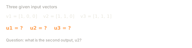
v1 = Vector([1, 0, 0])
v2 = Vector([1, 1, 0])
v3 = Vector([1, 1, 1])
basis = gram_schmidt([v1, v2, v3])
for i, u in enumerate(basis):
    print(f"u{i+1} = {u}")
    print(f"  |u{i+1}| = {u.magnitude():.6f}")

print(f"u1 · u2 = {basis[0].dot(basis[1]):.6f}")
print(f"u1 · u3 = {basis[0].dot(basis[2]):.6f}")
print(f"u2 · u3 = {basis[1].dot(basis[2]):.6f}")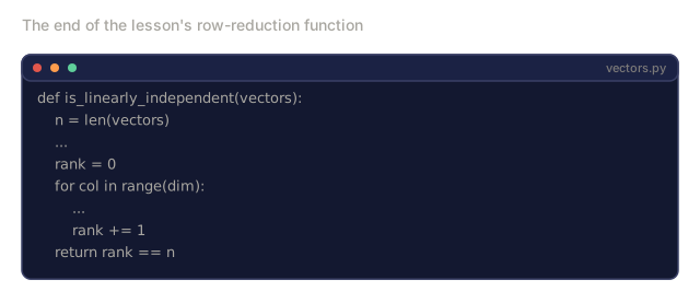
Use It
Now the same thing with NumPy, the version you'll actually use in practice:
import numpy as np

a = np.array([1, 2, 3], dtype=float)
b = np.array([4, 5, 6], dtype=float)

print(f"a + b = {a + b}")
print(f"a · b = {np.dot(a, b)}")
print(f"|a| = {np.linalg.norm(a):.4f}")
print(f"cosine = {np.dot(a, b) / (np.linalg.norm(a) * np.linalg.norm(b)):.4f}")

W = np.random.randn(2, 3) * 0.1
x = np.array([1.0, 0.5, -0.3])
print(f"Wx = {W @ x}")
Rank, Projection, and QR with NumPy
You already computed rank and projection by hand. NumPy gives you the same answers without the row-reduction loop, and this is the version you'll actually call in real code:
import numpy as np

A = np.array([[1, 2], [2, 4]])
print(f"Rank: {np.linalg.matrix_rank(A)}")

a = np.array([3, 4])
b = np.array([1, 0])
proj = (np.dot(a, b) / np.dot(b, b)) * b
print(f"Projection of {a} onto {b}: {proj}")

Q, R = np.linalg.qr(np.random.randn(3, 3))
print(f"Q is orthogonal: {np.allclose(Q @ Q.T, np.eye(3))}")
print(f"R is upper triangular: {np.allclose(R, np.triu(R))}")
PyTorch: Tensors Are Vectors with Autodiff
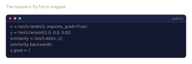
PyTorch's autodiff tracks every operation performed on a tensor, then computes the gradient of any downstream value with respect to that tensor, automatically. Training a neural network needs exactly this: how the output changes as each weight changes, for every weight, at every step. Deriving that by hand is what backpropagation was invented to avoid. Here's autodiff computing one gradient directly:
import torch

x = torch.randn(3, requires_grad=True)
y = torch.tensor([1.0, 0.0, 0.0])

similarity = torch.dot(x, y)
similarity.backward()

print(f"x = {x.data}")
print(f"y = {y.data}")
print(f"dot product = {similarity.item():.4f}")
print(f"d(dot)/dx = {x.grad}")
The gradient of the dot product with respect to x is just y. PyTorch computed this automatically. Every operation in a neural network is built from pieces like this: matrix multiplies, dot products, projections. Autodiff tracks gradients through all of them.
You just built from scratch what NumPy does in one line. Now you know what's happening under the hood.
Ship It
This lesson produces:
outputs/prompt-linear-algebra-tutor.md, a prompt for AI assistants to teach linear algebra through geometric intuition
Connections
Everything in this lesson connects to specific parts of modern AI:
| Concept | Where it shows up |
|---|---|
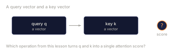
| Dot product | Attention scores in transformers, cosine similarity in RAG |
| Matrix multiply | Every neural network layer, every linear transformation |
| Linear independence | Feature selection, avoiding multicollinearity |
| Rank | Determining if a system is solvable, LoRA (low-rank adaptation) |
| Projection | Linear regression (projecting onto column space), PCA |
| Gram-Schmidt / QR | Numerical solvers, eigenvalue computation |
| Orthonormal basis | Stable numerical computation, whitening transforms |
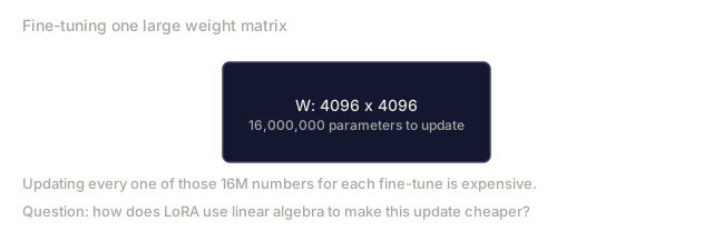
LoRA deserves special mention. It fine-tunes large language models by decomposing weight updates into low-rank matrices. Instead of updating a 4096x4096 weight matrix (16M parameters), LoRA updates two matrices of size 4096x16 and 16x4096 (131K parameters). The rank-16 constraint means LoRA assumes the weight update lives in a 16-dimensional subspace of the full 4096-dimensional space. That is linear algebra doing real work.

The subsection I see people skim past is Gram-Schmidt, and it's the one that comes back to bite you later. Nobody hand-runs Gram-Schmidt in production, but the moment you hit a numerically unstable least-squares solve, or wonder why np.linalg.qr even exists, this is the mechanism sitting underneath it.
Eigenvectors are the other one. The widget above looks like a toy until you're staring at a PCA plot or a spectral clustering result and need to know why it drew the axes it drew, not some other set.
If you already covered this material in a linear algebra course, don't skip the Build It section anyway. Writing the row-reduction loop by hand once is what turns np.linalg.matrix_rank from a black box you trust into a function whose answer you can predict before you run it.
Exercises
- Implement
Vector.angle_between(other)that returns the angle in degrees between two vectors - Create a 2D scaling matrix that doubles the x-coordinate and triples the y-coordinate, then apply it to the vector [1, 1]
- Given 5 random word-like vectors (dimension 50), find the two most similar using cosine similarity
- Verify that the Gram-Schmidt output is truly orthonormal: check that every pair has dot product 0 and every vector has magnitude 1
- Create a 3x3 matrix with rank 2. Verify using the
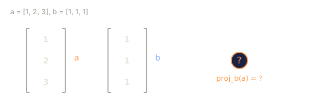
rank()method. Then explain what geometric object the columns span. - Project the vector [1, 2, 3] onto [1, 1, 1]. What does the result represent geometrically?
Key Terms
| Term | What people say | What it actually means |
|---|---|---|
| Vector | "An arrow" | A list of numbers representing a point or direction in n-dimensional space |
| Matrix | "A table of numbers" | A transformation that maps vectors from one space to another |
| Dot product | "Multiply and sum" | A measure of how aligned two vectors are: the core of similarity search |
| Embedding | "Some AI magic" | A vector that represents the meaning of something (word, image, user) |
| Linear independence | "They don't overlap" | No vector in the set can be written as a combination of the others |
| Rank | "How many dimensions" | The number of linearly independent columns (or rows) in a matrix |
| Projection | "The shadow" | The component of one vector in the direction of another |
| Basis | "The coordinate axes" | A minimal set of independent vectors that span the space |
| Orthonormal | "Perpendicular unit vectors" | Vectors that are mutually perpendicular and each have length 1 |
Code
- vectors.jl (text, 32 lines)
- vectors.py (python, 212 lines)