Embeddings & Vector Representations
Embeddings turn text into vectors so that meaning, not spelling, decides what counts as similar. Search, retrieval, and reranking all sit on that one idea, and this lesson builds the whole pipeline in plain numpy before pointing it at a real model.
Learning Objectives
- Generate text embeddings using API providers and open-source models, and compute cosine similarity between them
- Explain why embeddings solve the vocabulary mismatch problem that keyword search cannot handle
- Build a semantic search index that retrieves documents by meaning rather than exact keyword match
- Evaluate embedding quality using retrieval benchmarks (precision@k, recall) and choose the right embedding model for your task
The Problem
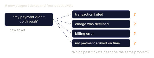
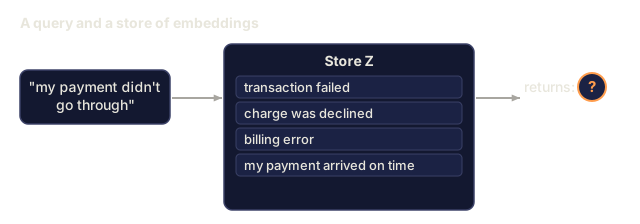
You have 10,000 support tickets. A customer writes "my payment didn't go through." You need to find similar past tickets. Keyword search finds tickets containing "payment" and "didn't go through." It misses "transaction failed," "charge was declined," and "billing error." These tickets describe the exact same problem in different words.
This is the vocabulary mismatch problem. Human language has dozens of ways to say the same thing. Keyword search treats each word as an independent symbol with no meaning. It cannot know that "declined" and "didn't go through" refer to the same concept.
You need a representation of text where meaning, not spelling, determines similarity. You need a way to place "my payment didn't go through" and "transaction was declined" close together in some mathematical space, while pushing "my payment arrived on time" far away despite sharing the word "payment."
That representation is an embedding.
The Concept
What Is an Embedding?
An embedding is a dense vector of floating-point numbers that represents the meaning of text. The word "dense" matters: every dimension carries information, unlike sparse representations (bag-of-words, TF-IDF) where most dimensions are zero.
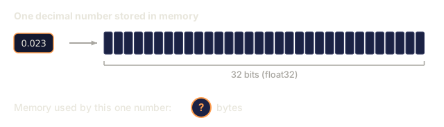
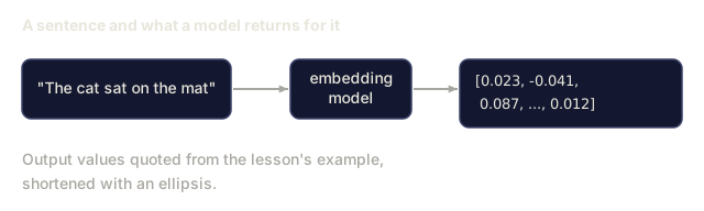
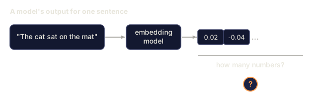
"The cat sat on the mat" becomes something like [0.023, -0.041, 0.087, ..., 0.012], a list of 768 to 3072 numbers depending on the model. These numbers encode meaning. You never inspect them directly. You compare them.
The Word2Vec Breakthrough
In 2013, Tomas Mikolov and colleagues at Google published Word2Vec. The core insight: train a neural network to predict a word from its neighbors (or neighbors from a word), and the hidden layer weights become meaningful vector representations.
The famous result:
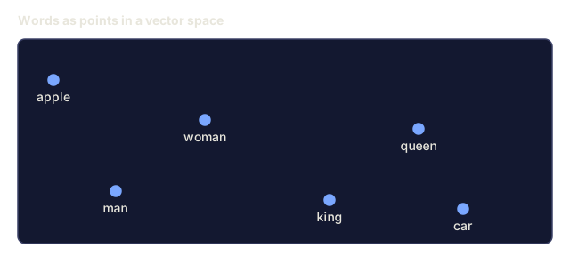
king - man + woman = queen
Vector arithmetic on word embeddings captures semantic relationships. The direction from "man" to "woman" is roughly the same as the direction from "king" to "queen." This was the moment the field realized that geometry could encode meaning.
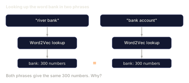
Word2Vec produced 300-dimensional vectors. Each word got one vector regardless of context. "Bank" in "river bank" and "bank account" had the same embedding. This limitation drove the next decade of research.
From Words to Sentences
Word embeddings represent single tokens. Production systems need to embed entire sentences, paragraphs, or documents. Four approaches emerged:
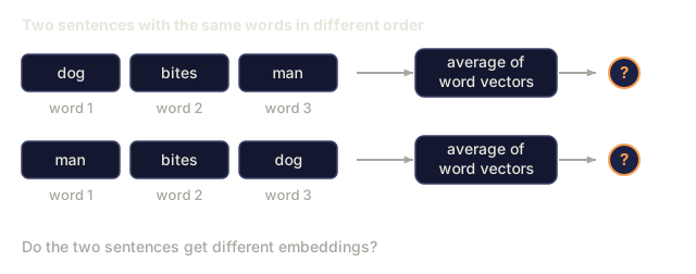
Averaging: take the mean of all word vectors in the sentence. Cheap, lossy, and decent for short text. Word order is lost, so "dog bites man" and "man bites dog" get identical embeddings.
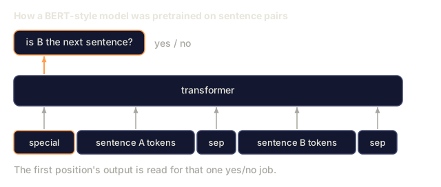
CLS token: transformer models (BERT, 2018) output a special [CLS] token embedding that represents the entire input. Better than averaging but the [CLS] token was trained for next-sentence prediction, not similarity.
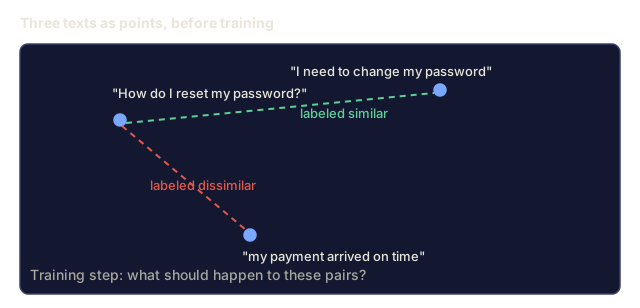
Contrastive learning: train the model explicitly to push similar pairs together and dissimilar pairs apart. Sentence-BERT (Reimers & Gurevych, 2019) used this approach and became the foundation for modern embedding models. Given "How do I reset my password?" and "I need to change my password," the model learns these should have nearly identical vectors.
Instruction-tuned embeddings: the latest approach. Models like E5 and GTE accept a task prefix ("search_query:", "search_document:") that tells the model what kind of embedding to produce. This lets one model serve multiple tasks.

Modern Embedding Models
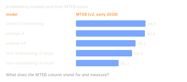
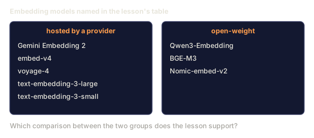
The market has settled into a handful of production-grade options (MTEB scores as of early 2026, MTEB v2):
| Model | Provider | Dimensions | MTEB | Context | Cost / 1M tokens |
|---|---|---|---|---|---|
| Gemini Embedding 2 | 3072 (Matryoshka) | 67.7 (retrieval) | 8192 | $0.15 | |
| embed-v4 | Cohere | 1024 (Matryoshka) | 65.2 | 128K | $0.12 |
| voyage-4 | Voyage AI | 1024/2048 (Matryoshka) | 66.8 | 32K | $0.12 |
| text-embedding-3-large | OpenAI | 3072 (Matryoshka) | 64.6 | 8192 | $0.13 |
| text-embedding-3-small | OpenAI | 1536 (Matryoshka) | 62.3 | 8192 | $0.02 |
| BGE-M3 | BAAI | 1024 (dense+sparse+ColBERT) | 63.0 multilingual | 8192 | Open-weight |
| Qwen3-Embedding | Alibaba | 4096 (Matryoshka) | 66.9 | 32K | Open-weight |
| Nomic-embed-v2 | Nomic | 768 (Matryoshka) | 63.1 | 8192 | Open-weight |
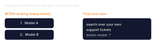
MTEB (Massive Text Embedding Benchmark) v2 covers 100+ tasks across retrieval, classification, clustering, reranking, and summarization. Higher is better. By 2026, open-weight models (Qwen3-Embedding, BGE-M3) match or beat closed hosted models on most axes. Gemini Embedding 2 leads pure retrieval; Voyage/Cohere lead specific domains (finance, law, code). Benchmark on your own queries before committing.
Similarity Metrics
Given two embedding vectors, three ways to measure how similar they are:
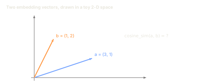
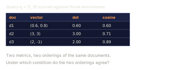
Cosine similarity: the cosine of the angle between two vectors. Ranges from -1 (opposite) to 1 (identical direction). Ignores magnitude, so a 10-word sentence and a 500-word document can score 1.0 if they point the same direction. This is the default for 90% of use cases.
cosine_sim(a, b) = dot(a, b) / (||a|| * ||b||)
Dot product: the raw inner product of two vectors. Identical to cosine similarity when vectors are normalized (unit length). Faster to compute. OpenAI's embeddings are normalized, so dot product and cosine give the same ranking.
dot(a, b) = sum(a_i * b_i)
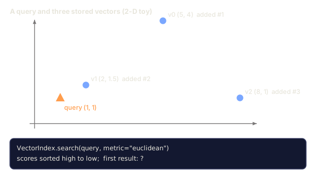
Euclidean (L2) distance: straight-line distance in the vector space. Smaller means more similar. Sensitive to magnitude differences. Use when the absolute position in space matters, not just the direction.
L2(a, b) = sqrt(sum((a_i - b_i)^2))
When to use which:
| Metric | Use when | Avoid when |
|---|---|---|
| Cosine similarity | Comparing texts of different lengths; most retrieval tasks | Magnitude carries information |
| Dot product | Embeddings are already normalized; maximum speed | Vectors have varying magnitudes |
| Euclidean distance | Clustering; spatial nearest-neighbor problems | Comparing documents of wildly different lengths |
Vector Databases and HNSW
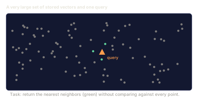
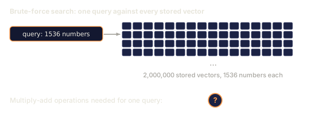
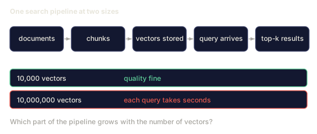
A brute-force similarity search compares the query against every stored vector. At 1 million vectors with 1536 dimensions, that is 1.5 billion multiply-add operations per query. Too slow.
Vector databases solve this with Approximate Nearest Neighbor (ANN) algorithms. The dominant algorithm is HNSW (Hierarchical Navigable Small World):
- Build a multi-layer graph of vectors
- Top layers are sparse, with long-range connections between distant clusters
- Bottom layers are dense, with fine-grained connections between nearby vectors
- Search starts at the top layer, greedily descending to refine
- Returns approximate top-k results in O(log n) time instead of O(n)
HNSW trades a small accuracy loss (typically 95-99% recall) for massive speed gains. At 10 million vectors, brute force takes seconds. HNSW takes milliseconds.

Production options:
| Database | Type | Best for | Max scale |
|---|---|---|---|
| Pinecone | Managed SaaS | Zero-ops production | Billions |
| Weaviate | Open source | Self-hosted, hybrid search | 100M+ |
| Qdrant | Open source | High performance, filtering | 100M+ |
| ChromaDB | Embedded | Prototyping, local dev | 1M |
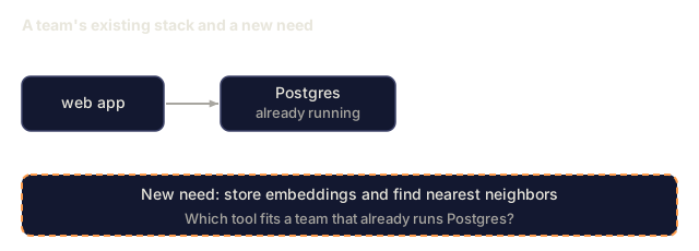
| pgvector | Postgres extension | Already using Postgres | 10M |
| FAISS | Library | In-process, research | 1B+ |
Chunking Strategies
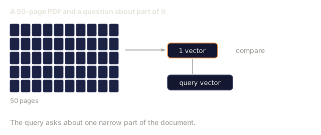
Documents are too long to embed as single vectors. A 50-page PDF covers dozens of topics, so its embedding becomes an average of everything, similar to nothing specific. You split documents into chunks and embed each one.
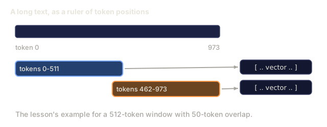
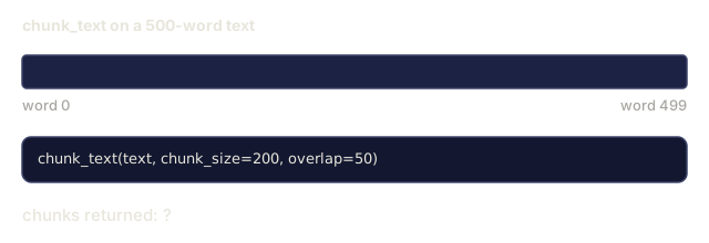
Fixed-size chunking: split every N tokens with M-token overlap. Simple and predictable. Works well when documents have no clear structure. A 512-token chunk with 50-token overlap: chunk 1 is tokens 0-511, chunk 2 is tokens 462-973.
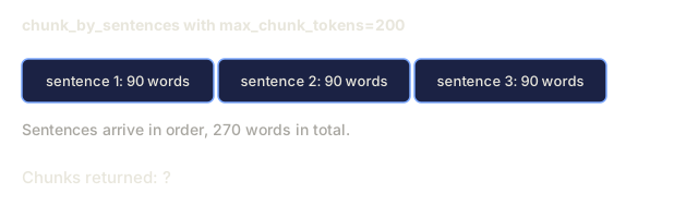
Sentence-based chunking: split at sentence boundaries, grouping sentences until reaching the token limit. Each chunk is at least one complete sentence. Better than fixed-size because you never cut a thought in half.
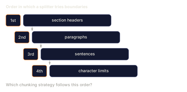
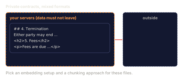
Recursive chunking: try splitting at the largest boundary first (section headers). If still too large, try paragraph boundaries. Then sentence boundaries. Then character limits. This is LangChain's RecursiveCharacterTextSplitter and it works well for mixed-format corpora.
Semantic chunking: embed each sentence, then group consecutive sentences whose embeddings are similar. When the embedding similarity drops below a threshold, start a new chunk. Expensive (requires embedding every sentence individually) but produces the most coherent chunks.
| Strategy | Complexity | Quality | Best for |
|---|---|---|---|
| Fixed-size | Low | Decent | Unstructured text, logs |
| Sentence-based | Low | Good | Articles, emails |
| Recursive | Medium | Good | Markdown, HTML, mixed docs |
| Semantic | High | Best | Critical retrieval quality |
The sweet spot for most systems: 256-512 token chunks with 50-token overlap.
Bi-Encoders vs Cross-Encoders
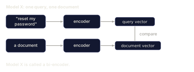
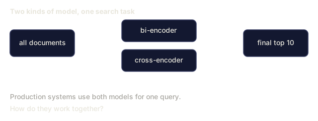
A bi-encoder embeds the query and documents independently, then compares vectors. Fast: you embed the query once and compare against pre-computed document embeddings. This is what you use for retrieval.
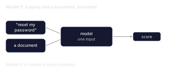
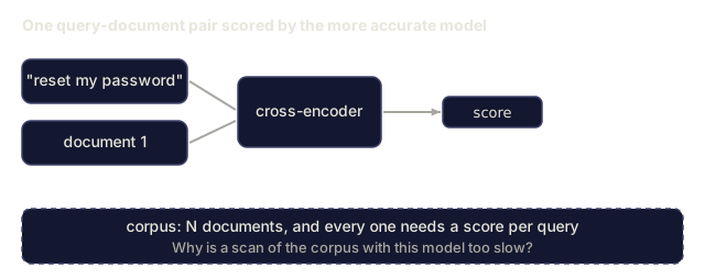
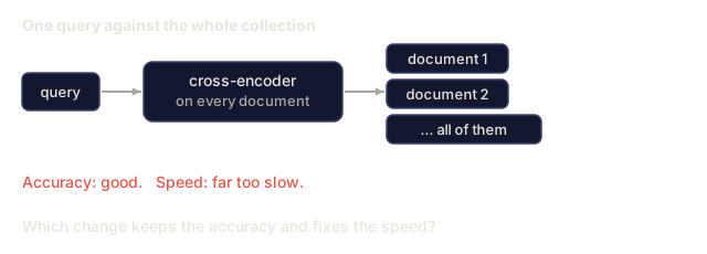
A cross-encoder takes the query and a document as a single input and outputs a relevance score. Slow, because it processes each query-document pair through the full model. But far more accurate because it can attend across query and document tokens simultaneously.
The production pattern: bi-encoder retrieves top-100 candidates, cross-encoder reranks them to top-10. This is the retrieve-then-rerank pipeline.

Reranking models: Cohere Rerank 3.5 ($2 per 1000 queries), BGE-reranker-v2 (free, open source), Jina Reranker v2 (free, open source).
Matryoshka Embeddings
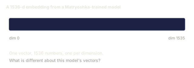
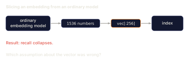
Traditional embeddings are all-or-nothing. A 1536-dimensional vector uses 1536 floats. You cannot truncate to 256 dimensions without retraining.
Matryoshka Representation Learning (Kusupati et al., 2022) fixes this. The model is trained so that the first N dimensions capture the most important information, like a Russian nesting doll. Truncating a 1536-d Matryoshka embedding to 256 dimensions loses some accuracy but remains functional.
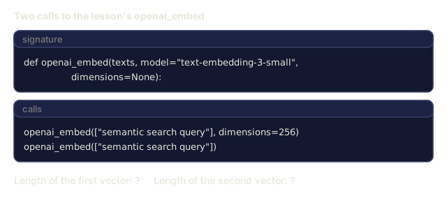
OpenAI's text-embedding-3-small and text-embedding-3-large support Matryoshka truncation via the dimensions parameter. Requesting 256 dimensions instead of 1536 cuts storage by 6x with roughly 3-5% accuracy loss on MTEB benchmarks.
Binary Quantization
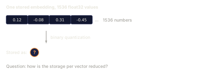
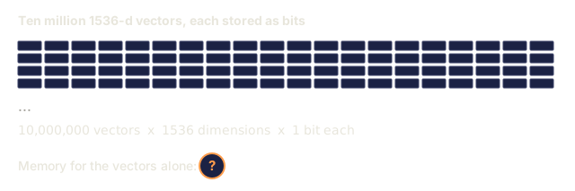
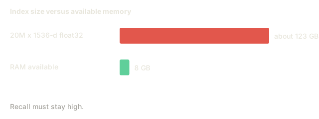
A 1536-dimensional embedding stored as float32 uses 6,144 bytes. Multiply by 10 million documents: 61 GB just for vectors.
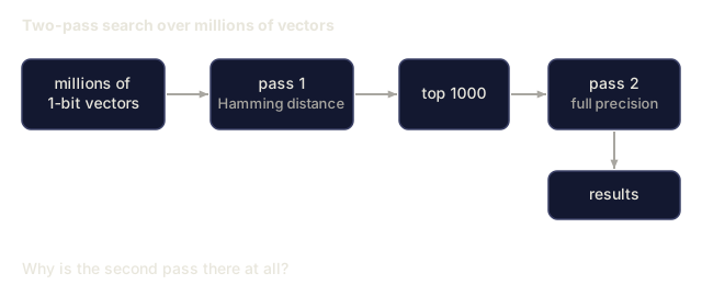
Binary quantization converts each float to a single bit: positive values become 1, negative values become 0. Storage drops from 6,144 bytes to 192 bytes, a 32x reduction. Similarity is computed using Hamming distance (count differing bits), which CPUs can do in a single instruction.
The accuracy hit is around 5-10% on retrieval recall. The common pattern: binary quantization for the first-pass search over millions of vectors, then rescore the top-1000 with full-precision vectors. This gets you 95%+ of full-precision accuracy at 32x less memory.
Build It
We build a semantic search engine from scratch. No vector database. No external embedding API. Pure Python with numpy for the math.
Step 1: Text Chunking
def chunk_text(text, chunk_size=200, overlap=50):
    words = text.split()
    chunks = []
    start = 0
    while start < len(words):
        end = start + chunk_size
        chunk = " ".join(words[start:end])
        chunks.append(chunk)
        start += chunk_size - overlap
    return chunks


def chunk_by_sentences(text, max_chunk_tokens=200):
    sentences = text.replace("\n", " ").split(".")
    sentences = [s.strip() + "." for s in sentences if s.strip()]
    chunks = []
    current_chunk = []
    current_length = 0
    for sentence in sentences:
        sentence_length = len(sentence.split())
        if current_length + sentence_length > max_chunk_tokens and current_chunk:
            chunks.append(" ".join(current_chunk))
            current_chunk = []
            current_length = 0
        current_chunk.append(sentence)
        current_length += sentence_length
    if current_chunk:
        chunks.append(" ".join(current_chunk))
    return chunks
Step 2: Building Embeddings from Scratch
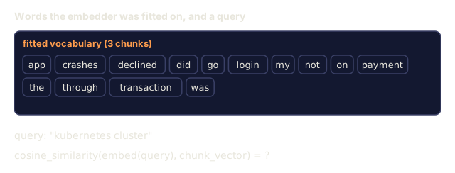
We implement a simple dense embedding using TF-IDF with L2 normalization. This is not a neural embedding, but it follows the same contract: text in, fixed-size vector out, similar texts produce similar vectors.
import math
import numpy as np
from collections import Counter

class SimpleEmbedder:
    def __init__(self):
        self.vocab = []
        self.idf = []
        self.word_to_idx = {}

    def fit(self, documents):
        vocab_set = set()
        for doc in documents:
            vocab_set.update(doc.lower().split())
        self.vocab = sorted(vocab_set)
        self.word_to_idx = {w: i for i, w in enumerate(self.vocab)}
        n = len(documents)
        self.idf = np.zeros(len(self.vocab))
        for i, word in enumerate(self.vocab):
            doc_count = sum(1 for doc in documents if word in doc.lower().split())
            self.idf[i] = math.log((n + 1) / (doc_count + 1)) + 1

    def embed(self, text):
        words = text.lower().split()
        count = Counter(words)
        total = len(words) if words else 1
        vec = np.zeros(len(self.vocab))
        for word, freq in count.items():
            if word in self.word_to_idx:
                tf = freq / total
                vec[self.word_to_idx[word]] = tf * self.idf[self.word_to_idx[word]]
        norm = np.linalg.norm(vec)
        if norm > 0:
            vec = vec / norm
        return vec
Step 3: Similarity Functions
def cosine_similarity(a, b):
    dot = np.dot(a, b)
    norm_a = np.linalg.norm(a)
    norm_b = np.linalg.norm(b)
    if norm_a == 0 or norm_b == 0:
        return 0.0
    return float(dot / (norm_a * norm_b))


def dot_product(a, b):
    return float(np.dot(a, b))


def euclidean_distance(a, b):
    return float(np.linalg.norm(a - b))
Step 4: Vector Index with Brute-Force Search
class VectorIndex:
    def __init__(self):
        self.vectors = []
        self.texts = []
        self.metadata = []

    def add(self, vector, text, meta=None):
        self.vectors.append(vector)
        self.texts.append(text)
        self.metadata.append(meta or {})

    def search(self, query_vector, top_k=5, metric="cosine"):
        scores = []
        for i, vec in enumerate(self.vectors):
            if metric == "cosine":
                score = cosine_similarity(query_vector, vec)
            elif metric == "dot":
                score = dot_product(query_vector, vec)
            elif metric == "euclidean":
                score = -euclidean_distance(query_vector, vec)
            else:
                raise ValueError(f"Unknown metric: {metric}")
            scores.append((i, score))
        scores.sort(key=lambda x: x[1], reverse=True)
        results = []
        for idx, score in scores[:top_k]:
            results.append({
                "text": self.texts[idx],
                "score": score,
                "metadata": self.metadata[idx],
                "index": idx
            })
        return results

    def size(self):
        return len(self.vectors)
Step 5: The Semantic Search Engine
class SemanticSearchEngine:
    def __init__(self, chunk_size=200, overlap=50):
        self.embedder = SimpleEmbedder()
        self.index = VectorIndex()
        self.chunk_size = chunk_size
        self.overlap = overlap

    def index_documents(self, documents, source_names=None):
        all_chunks = []
        all_sources = []
        for i, doc in enumerate(documents):
            chunks = chunk_text(doc, self.chunk_size, self.overlap)
            all_chunks.extend(chunks)
            name = source_names[i] if source_names else f"doc_{i}"
            all_sources.extend([name] * len(chunks))
        self.embedder.fit(all_chunks)
        for chunk, source in zip(all_chunks, all_sources):
            vec = self.embedder.embed(chunk)
            self.index.add(vec, chunk, {"source": source})
        return len(all_chunks)

    def search(self, query, top_k=5, metric="cosine"):
        query_vec = self.embedder.embed(query)
        return self.index.search(query_vec, top_k, metric)

    def search_with_scores(self, query, top_k=5):
        results = self.search(query, top_k)
        return [
            {
                "text": r["text"][:200],
                "source": r["metadata"].get("source", "unknown"),
                "score": round(r["score"], 4)
            }
            for r in results
        ]
Step 6: Comparing Similarity Metrics
def compare_metrics(engine, query, top_k=3):
    results = {}
    for metric in ["cosine", "dot", "euclidean"]:
        hits = engine.search(query, top_k=top_k, metric=metric)
        results[metric] = [
            {"score": round(h["score"], 4), "preview": h["text"][:80]}
            for h in hits
        ]
    return results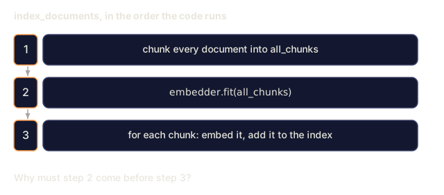
Use It
With a production embedding API, the architecture stays identical. Only the embedder changes:
from openai import OpenAI

client = OpenAI()

def openai_embed(texts, model="text-embedding-3-small", dimensions=None):
    kwargs = {"model": model, "input": texts}
    if dimensions:
        kwargs["dimensions"] = dimensions
    response = client.embeddings.create(**kwargs)
    return [item.embedding for item in response.data]
Matryoshka truncation with OpenAI (same model, fewer dimensions, lower storage):
full = openai_embed(["semantic search query"], dimensions=1536)
compact = openai_embed(["semantic search query"], dimensions=256)
The 256-d vector uses 6x less storage. For 10 million documents, that is 10 GB vs 61 GB. The accuracy loss is roughly 3-5% on standard benchmarks.
For reranking with Cohere:
import cohere

co = cohere.ClientV2()

results = co.rerank(
    model="rerank-v3.5",
    query="What is the refund policy?",
    documents=["Full refund within 30 days...", "No refunds after 90 days..."],
    top_n=3
)
For local embeddings with no API dependency:
from sentence_transformers import SentenceTransformer

model = SentenceTransformer("BAAI/bge-small-en-v1.5")
embeddings = model.encode(["semantic search query", "another document"])
The VectorIndex class from our build works with any of these. Swap the embedding function, keep the search logic.
Ship It
This lesson produces:
outputs/prompt-embedding-advisor.md: a prompt for choosing embedding models and strategies for specific use casesoutputs/skill-embedding-patterns.md: a skill that teaches agents how to use embeddings effectively in production
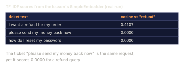
I'd run embeddings.py and read the similarity comparison (STEP 3 in its printed output) before anything else. SimpleEmbedder is TF-IDF over a vocabulary built from the corpus, so it only sees spelling. "Payment transaction was declined by the bank" and "My credit card charge did not go through" share no words, and the script prints a cosine of 0.0000 for the pair. That number is the vocabulary mismatch problem from The Problem, measured. It is also the reason a neural embedding exists.
The two production tricks in the file are simulations, and they behave like it. truncate_embedding slices the first N entries of a vector whose dimensions are the alphabetically sorted vocabulary, so cutting it drops words, not the least important directions. Matryoshka training is what makes real truncation work, and nothing here does that. In the same way, binarize is vec > 0 on non-negative TF-IDF weights, so it keeps only which words appear. On the sample corpus the "API rate limits" query shares 1 of 5 top results between cosine and Hamming search. I wouldn't read that as what binary quantization does to a real embedding.
The part that carries over is the shape. VectorIndex scans every stored vector on every query, which is the cost HNSW exists to avoid, and it takes any vector you hand it. Swap SimpleEmbedder for one of the models in Use It and the search logic stays as written. That swap is where I'd start the exercises.
Exercises
-
Metric comparison: run the same 5 queries against the sample documents using cosine similarity, dot product, and euclidean distance. Record the top-3 results for each. For which queries do the metrics disagree? Why?
-
Chunk size experiment: index the sample documents with chunk sizes of 50, 100, 200, and 500 words. For each, run 5 queries and record the top-1 similarity score. Plot the relationship between chunk size and retrieval quality. Find the point where larger chunks start hurting.
-
Matryoshka simulation: build a SimpleEmbedder that produces 500-d vectors. Truncate to 50, 100, 200, and 500 dimensions. Measure how retrieval recall degrades at each truncation. This simulates Matryoshka behavior without needing the real training trick.
-
Binary quantization: take the embeddings from the search engine, convert them to binary (1 if positive, 0 if negative), and implement Hamming distance search. Compare the top-10 results against full-precision cosine similarity. Measure the overlap percentage.
-
Sentence-based chunking: replace fixed-size chunking with
chunk_by_sentences. Run the same queries and compare retrieval scores. Does respecting sentence boundaries improve the results?
Key Terms
| Term | What people say | What it actually means |
|---|---|---|
| Embedding | "Text to numbers" | A dense vector where geometric proximity encodes semantic similarity |
| Word2Vec | "The OG embedding" | 2013 model that learned word vectors by predicting context words; proved vector arithmetic encodes meaning |
| Cosine similarity | "How similar are two vectors" | Cosine of the angle between vectors; 1 = identical direction, 0 = orthogonal, -1 = opposite |
| HNSW | "Fast vector search" | Hierarchical Navigable Small World graph -- multi-layer structure enabling O(log n) approximate nearest neighbor search |
| Bi-encoder | "Embed separately, compare fast" | Encodes query and document independently into vectors; enables pre-computation and fast retrieval |
| Cross-encoder | "Slow but accurate reranker" | Processes query-document pair jointly through the full model; higher accuracy, no pre-computation |
| Matryoshka embeddings | "Truncatable vectors" | Embeddings trained so the first N dimensions capture the most important information, enabling variable-size storage |
| Binary quantization | "1-bit embeddings" | Converting float vectors to binary (sign bit only) for 32x storage reduction with Hamming distance search |
| Chunking | "Split docs for embedding" | Breaking documents into 256-512 token segments so each can be independently embedded and retrieved |
| Vector database | "Search engine for embeddings" | Data store optimized for storing vectors and performing approximate nearest neighbor search at scale |
| Contrastive learning | "Train by comparison" | Training approach that pushes similar pair embeddings together and dissimilar pair embeddings apart |
| MTEB | "The embedding benchmark" | Massive Text Embedding Benchmark -- 56 datasets across 8 tasks; standard for comparing embedding models |
Further Reading
- Mikolov et al., "Efficient Estimation of Word Representations in Vector Space" (2013): the Word2Vec paper that started the embedding revolution with the king-queen analogy
- Reimers & Gurevych, "Sentence-BERT: Sentence Embeddings using Siamese BERT-Networks" (2019): how to train bi-encoders for sentence-level similarity, foundation of modern embedding models
- Kusupati et al., "Matryoshka Representation Learning" (2022): the technique behind variable-dimension embeddings that OpenAI adopted for text-embedding-3
- Malkov & Yashunin, "Efficient and Robust Approximate Nearest Neighbor using Hierarchical Navigable Small World Graphs" (2018): the HNSW paper, the algorithm behind most production vector search
- OpenAI Embeddings Guide (platform.openai.com/docs/guides/embeddings): practical reference for text-embedding-3 models including Matryoshka dimension reduction
- MTEB Leaderboard (huggingface.co/spaces/mteb/leaderboard): live benchmark comparing all embedding models across tasks and languages
- Muennighoff et al., "MTEB: Massive Text Embedding Benchmark" (EACL 2023): the benchmark defining 8 task categories (classification, clustering, pair classification, reranking, retrieval, STS, summarization, bitext mining) that the leaderboard reports; read before trusting any single MTEB score.
- Sentence Transformers documentation: canonical reference for bi-encoder vs cross-encoder, pooling strategies, and the ingest-split-embed-store RAG pipeline this lesson implements. [ { "question": "What problem do embeddings solve that keyword search cannot?", "options": [ "Embeddings are faster", "Embeddings capture semantic meaning, matching 'payment didn't go through' with 'charge was declined' even though they share no words", "Embeddings use less storage", "Embeddings work offline" ], "correct": 1, "explanation": "Keyword search treats words as independent symbols. Embeddings map text to high-dimensional vectors where semantic similarity = geometric proximity. Texts with the same meaning cluster together regardless of word choice.", "stage": "pre" }, { "question": "What does cosine similarity measure between two embedding vectors?", "options": [ "The Euclidean distance", "The angle between the vectors, indicating how similar their directions are regardless of magnitude", "The sum of their components", "The number of matching dimensions" ], "correct": 1, "explanation": "Cosine similarity = dot(A,B) / (|A|*|B|). It ranges from -1 (opposite) to 1 (identical direction). Two texts with the same meaning will have vectors pointing in nearly the same direction, giving cosine similarity near 1.", "stage": "pre" }, { "question": "What is the typical dimensionality of modern text embedding models?", "options": [ "2-10 dimensions", "50-100 dimensions", "768-3072 dimensions", "100,000+ dimensions" ], "correct": 2, "explanation": "Modern embedding models (OpenAI text-embedding-3, BGE, E5) produce vectors with 768 to 3072 dimensions. Higher dimensions capture more nuance but cost more to store and search.", "stage": "post" }, { "question": "Why should you evaluate embedding quality using retrieval benchmarks rather than just inspecting similarity scores?", "options": [ "Similarity scores are always wrong", "Absolute similarity values vary by model; what matters is whether relevant documents rank higher than irrelevant ones (precision@k, recall)", "Retrieval benchmarks are faster", "Similarity scores don't use cosine distance" ], "correct": 1, "explanation": "A cosine similarity of 0.85 might mean 'very similar' for one model and 'somewhat similar' for another, since raw similarity scores aren't calibrated the same way across models. What matters is whether relevant documents actually rank above irrelevant ones, which is what retrieval benchmarks like MTEB measure directly.", "stage": "post" }, { "question": "When would you use a local/open-source embedding model instead of an API-based one?", "options": [ "Local models are always better", "When you need data privacy, offline operation, lower cost at scale, or domain-specific fine-tuning", "Local models produce higher quality embeddings", "API models don't support batching" ], "correct": 1, "explanation": "API embeddings (OpenAI, Cohere) are easy but send your data externally. Local models (BGE, E5, Nomic) keep data private, eliminate per-call costs at scale, and can be fine-tuned on domain-specific data.", "stage": "post" }, { "question": "What breakthrough did Word2Vec (Mikolov et al., 2013) demonstrate about word embeddings?", "options": [ "That embeddings must always have exactly 768 dimensions", "That keyword search outperforms semantic search for short queries", "That embeddings require labeled training data from crowdworkers", "That vector arithmetic on word embeddings captures semantic relationships, illustrated by king minus man plus woman equaling queen" ], "correct": 3, "explanation": "The lesson credits Word2Vec with the famous king - man + woman = queen result, showing the direction from man to woman roughly matches the direction from king to queen in vector space.", "stage": "check" }, { "question": "Of the four sentence-embedding approaches the lesson covers, which one uses a special transformer output token that was originally trained for next-sentence prediction rather than similarity?", "options": [ "Averaging", "CLS token", "Contrastive learning", "Instruction-tuned embeddings" ], "correct": 1, "explanation": "The lesson notes the CLS-token approach from transformer models like BERT is 'better than averaging but the [CLS] token was trained for next-sentence prediction, not similarity.'", "stage": "check" }, { "question": "How does HNSW (Hierarchical Navigable Small World) make vector search fast at scale, according to the lesson?", "options": [ "It builds a multi-layer graph where sparse top layers allow long-range jumps and dense bottom layers refine the search, returning approximate results in O(log n) instead of O(n)", "It deletes older vectors once the index reaches 1 million entries", "It compresses every vector to a single bit before comparing them", "It re-trains the embedding model on the query at search time" ], "correct": 0, "explanation": "The lesson describes HNSW as a multi-layer graph: searches start at sparse top layers and descend to dense bottom layers, trading a small accuracy loss for O(log n) search instead of brute-force O(n).", "stage": "check" }, { "question": "Per the lesson's vector database comparison table, which option is a Postgres extension best suited for teams already running Postgres?", "options": [ "Pinecone", "ChromaDB", "pgvector", "FAISS" ], "correct": 2, "explanation": "The lesson's table lists pgvector as a 'Postgres extension' best for teams 'already using Postgres,' scaling to roughly 10 million vectors.", "stage": "post" }, { "question": "Which chunking strategy does the lesson describe as trying section headers first, then paragraph boundaries, then sentence boundaries, then character limits?", "options": [ "Fixed-size chunking", "Sentence-based chunking", "Semantic chunking", "Recursive chunking" ], "correct": 3, "explanation": "The lesson defines recursive chunking as trying 'the largest boundary first (section headers)' and falling back through paragraphs, sentences, and character limits, citing LangChain's RecursiveCharacterTextSplitter as an example.", "stage": "check" }, { "question": "What production pattern does the lesson describe for combining bi-encoders and cross-encoders?", "options": [ "A bi-encoder retrieves a larger candidate set (for example, top-100), then a cross-encoder reranks it down to a smaller final set (for example, top-10)", "Use only cross-encoders, since bi-encoders are obsolete", "Run both independently and average their scores", "Use a bi-encoder for reranking after a cross-encoder narrows the candidates" ], "correct": 0, "explanation": "The lesson calls this the 'retrieve-then-rerank pipeline': a fast bi-encoder retrieves top-100 candidates, then a slower but more accurate cross-encoder reranks them down to top-10.", "stage": "check" }, { "question": "What makes Matryoshka embeddings different from traditional fixed embeddings, per the lesson?", "options": [ "They can only be generated by open-source models", "They double the vector's dimensionality automatically at query time", "They are trained so the first N dimensions carry the most important information, so truncating the vector still produces a usable, smaller embedding without retraining", "They eliminate the need for a similarity metric entirely" ], "correct": 2, "explanation": "The lesson compares Matryoshka embeddings to a nesting doll: the model is trained so the first N dimensions capture the most important information, letting a 1536-d vector truncate to 256 dimensions with only 3-5% accuracy loss.", "stage": "post" }, { "question": "How does binary quantization reduce vector storage, according to the lesson?", "options": [ "It deletes half of the stored vectors at random", "It stores vectors as compressed JPEG images", "It merges every two dimensions into one using averaging", "It converts each float in the embedding to a single bit (positive becomes 1, negative becomes 0), cutting a 6,144-byte vector down to 192 bytes, a 32x reduction" ], "correct": 3, "explanation": "The lesson describes binary quantization as converting each float to a single bit, shrinking a 1536-dimension float32 vector from 6,144 bytes to 192 bytes, searched afterward using Hamming distance.", "stage": "post" }, { "question": "According to the lesson, when does dot product similarity produce the same ranking as cosine similarity?", "options": [ "Only when using Euclidean distance instead", "When the vectors are normalized to unit length, as OpenAI's embeddings are, so dot product gives the same ranking as cosine similarity but computes faster", "Only when comparing exactly two vectors at a time", "Never; they always produce different rankings" ], "correct": 1, "explanation": "The lesson states dot product is 'identical to cosine similarity when vectors are normalized (unit length)' and notes OpenAI's embeddings are normalized, so the two metrics give the same ranking while dot product is faster to compute.", "stage": "check" }
Code
- embeddings.py (python, 418 lines)
- main.ts (typescript, 356 lines)