Singular Value Decomposition
Every matrix, of any shape or rank, factors into a rotation, a scale, and another rotation. No exceptions. Master that one decomposition and PCA, recommender systems, and least-squares regression stop looking like separate problems.
Learning Objectives
- Implement SVD via power iteration and explain the geometric meaning of U, Sigma, and V^T
- Apply truncated SVD for image compression and measure the compression ratio vs reconstruction error
- Compute the Moore-Penrose pseudoinverse via SVD to solve overdetermined least-squares systems
- Connect SVD to PCA, recommendation systems (latent factors), and Latent Semantic Analysis in NLP
The Problem
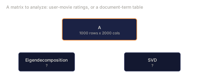
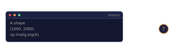
Say you're holding a 1000x2000 matrix: user-movie ratings, a document-term frequency table, or the pixel values of an image, it doesn't matter which. You need to compress it, denoise it, find the structure hiding inside it, or solve a least-squares system against it. Eigendecomposition can't help here. It only works on square matrices, and even then only when the matrix has a full set of linearly independent eigenvectors.
SVD carries none of those restrictions. Any matrix, any shape, any rank, factors into three pieces that expose exactly what the matrix does to space, geometrically. Nothing else in linear algebra generalizes this far.
The Concept
What SVD does geometrically
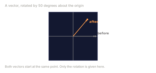
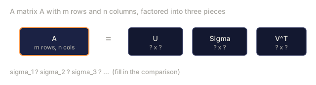
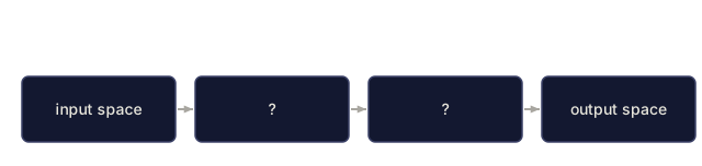
SVD factors any matrix A into three pieces, A = U * Sigma * V^T, that correspond to three geometric operations applied in sequence: rotate, scale, rotate. That holds regardless of the matrix's shape.
A = U * Sigma * V^T

      m x n     m x m    m x n    n x n
     (any)    (rotate)  (scale)  (rotate)
Given any matrix A, SVD factors it into:
- V^T rotates vectors in the input space (n-dimensional)
- Sigma scales along each axis (stretches or compresses)
- U rotates the result into the output space (m-dimensional)

Hand SVD a matrix and it hands back exactly what that matrix does to a sphere of inputs: first rotate it by V^T, then stretch it into an ellipsoid by Sigma, then rotate the ellipsoid by U. The singular values are the lengths of that ellipsoid's axes.
The full decomposition
For a matrix A with shape m x n:
A = U * Sigma * V^T

where:
  U     is m x m, orthogonal (U^T U = I)
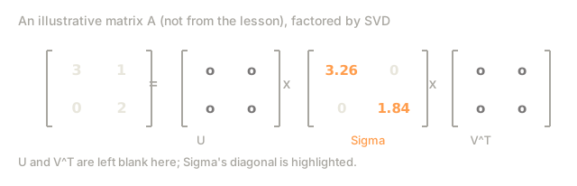
  Sigma is m x n, diagonal (singular values on the diagonal)
  V     is n x n, orthogonal (V^T V = I)

The singular values sigma_1 >= sigma_2 >= ... >= sigma_r > 0
where r = rank(A)
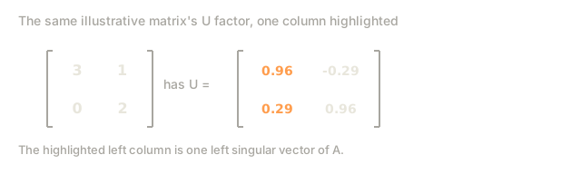
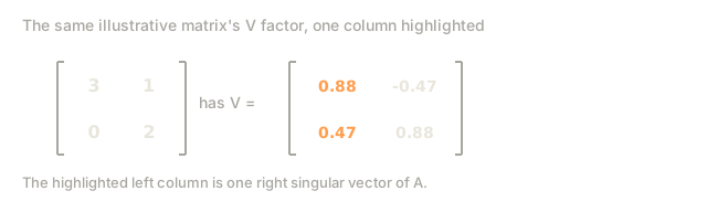
The columns of U are the left singular vectors, the columns of V are the right singular vectors, and the diagonal entries of Sigma are the singular values, which are always non-negative and sorted in decreasing order by convention.
Left singular vectors, singular values, right singular vectors
Each piece carries its own geometric job.
Right singular vectors (columns of V): an orthonormal basis for the input space (R^n), specifically the directions in that space the matrix sends to orthogonal directions on the output side. Treat them as the domain's natural coordinate system.
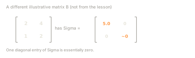
Singular values (diagonal of Sigma): the scaling factors. The i-th singular value says how much the matrix stretches vectors along the i-th right singular vector; a value of zero means that direction gets crushed entirely.
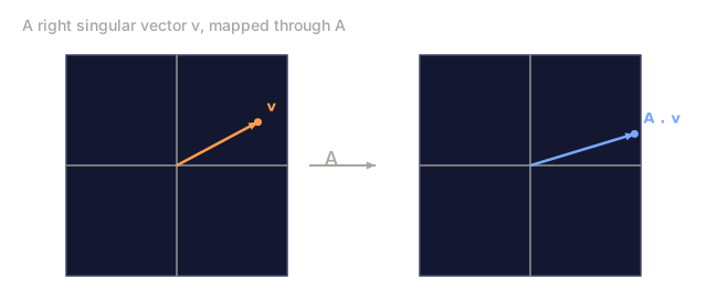
Left singular vectors (columns of U): an orthonormal basis for the output space (R^m). The i-th left singular vector is where the i-th right singular vector lands, once scaling has been applied.
One equation ties all three together:
A * v_i = sigma_i * u_i

The matrix A takes the i-th right singular vector v_i,
scales it by sigma_i, and maps it to the i-th left singular vector u_i.
Read coordinate by coordinate, that's the complete picture of what any matrix does.
Outer product form
The SVD can be written as a sum of rank-1 matrices:
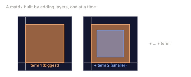
A = sigma_1 * u_1 * v_1^T + sigma_2 * u_2 * v_2^T + ... + sigma_r * u_r * v_r^T

Each term sigma_i * u_i * v_i^T is a rank-1 matrix (an outer product).
The full matrix is the sum of r such matrices, where r is the rank.
This form is the foundation of low-rank approximation: each term layers in one more pattern, ranked by importance, so the first captures the single most dominant structure and every term after adds a smaller correction on top. Truncate the sum early and you get the best possible approximation at that rank.
Rank-1 approx:    A_1 = sigma_1 * u_1 * v_1^T
                  (captures the dominant pattern)

Rank-2 approx:    A_2 = sigma_1 * u_1 * v_1^T + sigma_2 * u_2 * v_2^T
                  (captures the two most important patterns)

Rank-k approx:    A_k = sum of top k terms
                  (optimal by the Eckart-Young theorem)
Relationship to eigendecomposition
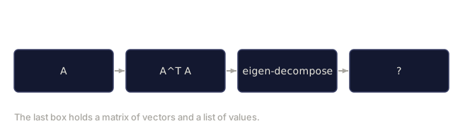
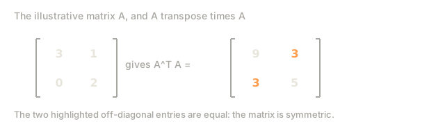
SVD and eigendecomposition are closely related: the singular values and vectors of A come directly from the eigenvalues and eigenvectors of A^T A and A A^T.
A^T A = V * Sigma^T * U^T * U * Sigma * V^T
      = V * Sigma^T * Sigma * V^T
      = V * D * V^T

where D = Sigma^T * Sigma is a diagonal matrix with sigma_i^2 on the diagonal.

So:
- The right singular vectors (V) are eigenvectors of A^T A
- The singular values squared (sigma_i^2) are eigenvalues of A^T A

Similarly:
A A^T = U * Sigma * V^T * V * Sigma^T * U^T
      = U * Sigma * Sigma^T * U^T

So:
- The left singular vectors (U) are eigenvectors of A A^T
- The eigenvalues of A A^T are also sigma_i^2
This connection tells you three things:
- Singular values are always real and non-negative, because they are square roots of eigenvalues of a positive semi-definite matrix: one whose eigenvalues never go negative, which A^T A always satisfies.
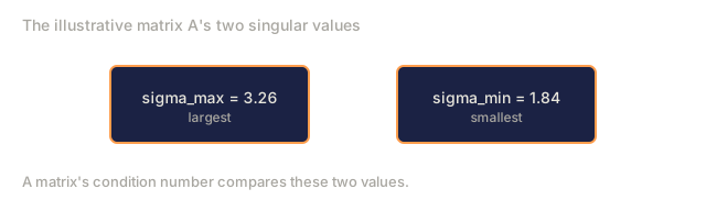
- You could compute SVD via eigendecomposition of A^T A, but that squares the condition number (the ratio between a matrix's largest and smallest singular value, which controls how much numerical error gets amplified) and loses numerical precision. Dedicated SVD algorithms avoid this.
- When A is square and symmetric positive semi-definite, SVD and eigendecomposition are the same thing.
Truncated SVD: low-rank approximation
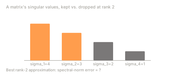
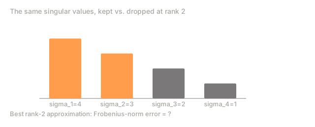
The Eckart-Young-Mirsky theorem states that the best rank-k approximation to A (in both Frobenius and spectral norm) is obtained by keeping only the top k singular values and their corresponding vectors:
A_k = U_k * Sigma_k * V_k^T

where:
  U_k     is m x k  (first k columns of U)
  Sigma_k is k x k  (top-left k x k block of Sigma)
  V_k     is n x k  (first k columns of V)

Approximation error = sigma_{k+1}  (in spectral norm)
                    = sqrt(sigma_{k+1}^2 + ... + sigma_r^2)  (in Frobenius norm)
Spectral norm measures that leftover error by its single largest singular value. Frobenius norm measures the same error by the square root of the sum of all its squared entries. Different rulers, same leftover.
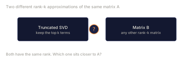
That's a provable optimum, not a rule of thumb: no other rank-k matrix sits closer to A than this one.
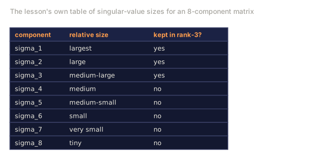
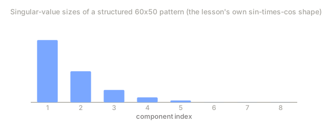
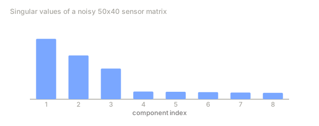
| Component | Relative magnitude | Kept in rank-3 approx? |
|---|---|---|
| sigma_1 | Largest | Yes |
| sigma_2 | Large | Yes |
| sigma_3 | Medium-large | Yes |
| sigma_4 | Medium | No (error) |
| sigma_5 | Medium-small | No (error) |
| sigma_6 | Small | No (error) |
| sigma_7 | Very small | No (error) |
| sigma_8 | Tiny | No (error) |
Keep top 3: A_3 captures the three largest singular values. Error = remaining values (sigma_4 through sigma_8).
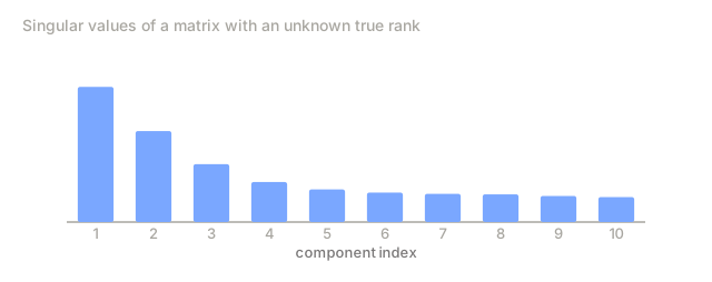
If singular values decay fast, a small k captures most of the matrix. If they decay slowly, the matrix has no low-rank structure.
Image compression with SVD
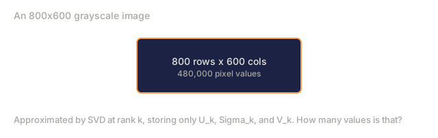
A grayscale image is a matrix of pixel intensities. An 800x600 image has 480,000 values. SVD lets you approximate it with far fewer.
Original image: 800 x 600 = 480,000 values

SVD with rank k:
  U_k:      800 x k values
  Sigma_k:  k values
  V_k:      600 x k values
  Total:    k * (800 + 600 + 1) = k * 1401 values

  k=10:   14,010 values   (2.9% of original)
  k=50:   70,050 values  (14.6% of original)
  k=100: 140,100 values  (29.2% of original)

  The compression ratio improves as k gets smaller,
  but visual quality degrades.
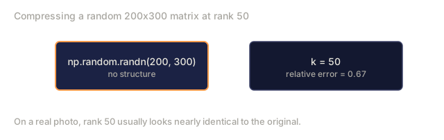
The key insight: natural images have rapidly decaying singular values. The first few capture broad structure, shapes and gradients; the later ones capture fine detail and noise. Truncating at rank 50 often produces an image nearly indistinguishable from the original while using 85% less storage.
SVD for recommendation systems
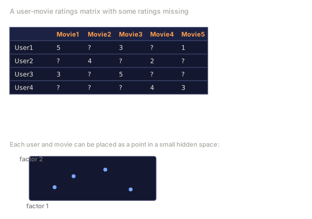
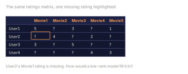
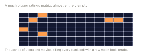
The Netflix Prize made this famous. You have a user-movie ratings matrix where most entries are missing.
             Movie1  Movie2  Movie3  Movie4  Movie5
  User1      [  5      ?       3       ?       1  ]
  User2      [  ?      4       ?       2       ?  ]
  User3      [  3      ?       5       ?       ?  ]
  User4      [  ?      ?       ?       4       3  ]

  ? = unknown rating
The idea: this ratings matrix has low rank, because users don't have completely independent tastes. A handful of latent factors (action vs. drama, old vs. new, cerebral vs. visceral) explain most of what any given user prefers.
SVD on the (filled-in) ratings matrix decomposes it into:
- U: user profiles in latent factor space
- Sigma: importance of each latent factor
- V^T: movie profiles in latent factor space
A user's predicted rating for a movie is the dot product of their user profile with the movie's profile (weighted by singular values). The low-rank approximation fills in the missing entries.
In practice, you use variants like Simon Funk's incremental SVD or ALS (alternating least squares) that handle missing data directly. But the core idea is the same: latent factor decomposition via SVD.
SVD in NLP: Latent Semantic Analysis
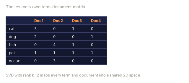
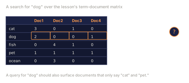
Latent Semantic Analysis (LSA), also called Latent Semantic Indexing (LSI), applies SVD to a term-document matrix.
             Doc1   Doc2   Doc3   Doc4
  "cat"      [  3      0      1      0  ]
  "dog"      [  2      0      0      1  ]
  "fish"     [  0      4      1      0  ]
  "pet"      [  1      1      1      1  ]
  "ocean"    [  0      3      0      0  ]

After SVD with rank k=2:

  Each document becomes a point in 2D "concept space."
  Each term becomes a point in the same 2D space.
  Documents about similar topics cluster together.
  Terms with similar meanings cluster together.

  "cat" and "dog" end up near each other (land pets).
  "fish" and "ocean" end up near each other (water concepts).
  Doc1 and Doc3 cluster if they share similar topics.
LSA was one of the first methods that actually worked for capturing semantic similarity from raw text. Synonymous terms tend to show up in similar documents, so SVD naturally groups them into the same latent dimensions. Modern word embeddings, Word2Vec, GloVe, descend from this same idea.
SVD for noise reduction
Noisy data has signal concentrated in the top singular values and noise spread across all singular values. Truncating removes the noise floor.
Clean signal singular values:
| Component | Magnitude | Type |
|---|---|---|
| sigma_1 | Very large | Signal |
| sigma_2 | Large | Signal |
| sigma_3 | Medium | Signal |
| sigma_4 | Near zero | Negligible |
| sigma_5 | Near zero | Negligible |
Noisy signal singular values (noise adds to all):
| Component | Magnitude | Type |
|---|---|---|
| sigma_1 | Very large | Signal |
| sigma_2 | Large | Signal |
| sigma_3 | Medium | Signal |
| sigma_4 | Small | Noise |
| sigma_5 | Small | Noise |
| sigma_6 | Small | Noise |
| sigma_7 | Small | Noise |

Signal processing, scientific measurement, data cleaning: any time a matrix is corrupted by additive noise, truncated SVD gives you a principled way to separate signal from noise.
Pseudoinverse via SVD
The Moore-Penrose pseudoinverse A+ generalizes matrix inversion to non-square and singular matrices. SVD makes computing it trivial.
If A = U * Sigma * V^T, then:

A+ = V * Sigma+ * U^T

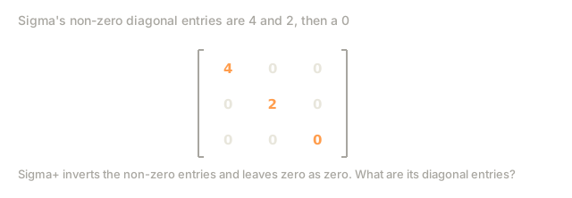
where Sigma+ is formed by:
  1. Transpose Sigma (swap rows and columns)
  2. Replace each non-zero diagonal entry sigma_i with 1/sigma_i
  3. Leave zeros as zeros

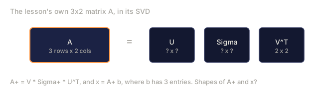
For A (m x n):      A+ is (n x m)
For Sigma (m x n):  Sigma+ is (n x m)
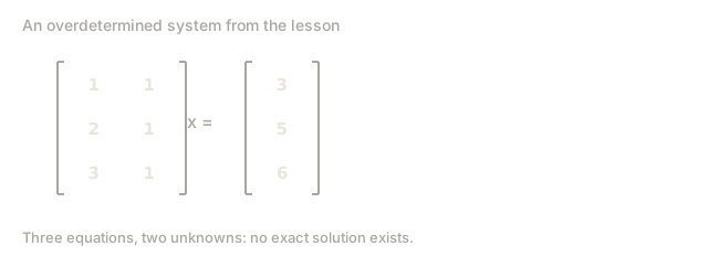
The pseudoinverse solves least-squares problems. If Ax = b has no exact solution (overdetermined system), then x = A+ b is the least-squares solution (minimizes ||Ax - b||).
Overdetermined system (more equations than unknowns):

  [1  1]         [3]
  [2  1] x   =   [5]       No exact solution exists.
  [3  1]         [6]

  x_ls = A+ b = V * Sigma+ * U^T * b

  This gives the x that minimizes the sum of squared residuals.
  Same result as the normal equations (A^T A)^(-1) A^T b,
  but numerically more stable.
Numerical stability advantages
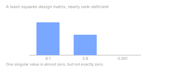
Computing eigendecomposition of A^T A squares the singular values (eigenvalues of A^T A are sigma_i^2). This squares the condition number, amplifying numerical errors.
Example:
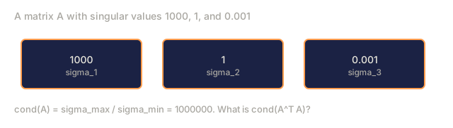
  A has singular values [1000, 1, 0.001]
  Condition number of A: 1000 / 0.001 = 10^6

  A^T A has eigenvalues [10^6, 1, 10^{-6}]
  Condition number of A^T A: 10^6 / 10^{-6} = 10^{12}

  Computing SVD directly: works with condition number 10^6
  Computing via A^T A:     works with condition number 10^{12}
                           (6 extra digits of precision lost)
Modern SVD algorithms (Golub-Kahan bidiagonalization) work directly on A, never forming A^T A. This is why you should always prefer np.linalg.svd(A) over np.linalg.eig(A.T @ A).
Connection to PCA
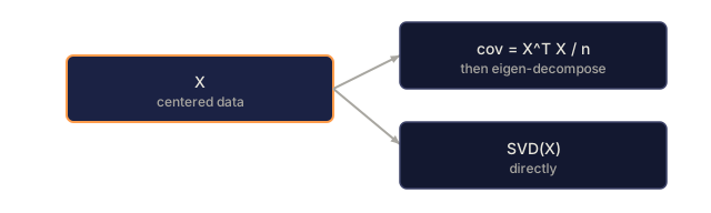
PCA IS SVD on centered data. Not an analogy: the literal same computation.
Given data matrix X (n_samples x n_features), centered (mean subtracted):

Covariance matrix: C = (1/(n-1)) * X^T X

PCA finds eigenvectors of C. But:

  X = U * Sigma * V^T    (SVD of X)

  X^T X = V * Sigma^2 * V^T

  C = (1/(n-1)) * V * Sigma^2 * V^T

So the principal components are exactly the right singular vectors V.
The explained variance for each component is sigma_i^2 / (n-1).

In sklearn, PCA is implemented using SVD, not eigendecomposition.
It is faster and more numerically stable.
Everything covered in Lesson 10 about dimensionality reduction is SVD under the hood, and PCA is SVD's most common application in machine learning.
Build It
Step 1: SVD from scratch using power iteration
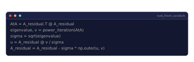
The idea: find the largest singular value and its vectors with power iteration on A^T A (or A A^T), then deflate the matrix and repeat for the next one.
import numpy as np

def power_iteration(M, num_iters=100):
    n = M.shape[1]
    v = np.random.randn(n)
    v = v / np.linalg.norm(v)

    for _ in range(num_iters):
        Mv = M @ v
        v = Mv / np.linalg.norm(Mv)

    eigenvalue = v @ M @ v
    return eigenvalue, v

def svd_from_scratch(A, k=None):
    m, n = A.shape
    if k is None:
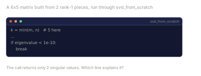
        k = min(m, n)

    sigmas = []
    us = []
    vs = []

    A_residual = A.copy().astype(float)

    for _ in range(k):
        AtA = A_residual.T @ A_residual
        eigenvalue, v = power_iteration(AtA, num_iters=200)

        if eigenvalue < 1e-10:
            break

        sigma = np.sqrt(eigenvalue)
        u = A_residual @ v / sigma

        sigmas.append(sigma)
        us.append(u)
        vs.append(v)

        A_residual = A_residual - sigma * np.outer(u, v)

    U = np.column_stack(us) if us else np.empty((m, 0))
    S = np.array(sigmas)
    V = np.column_stack(vs) if vs else np.empty((n, 0))

    return U, S, V
Step 2: Test and compare with NumPy
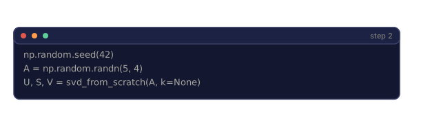
np.random.seed(42)
A = np.random.randn(5, 4)

U_ours, S_ours, V_ours = svd_from_scratch(A)
U_np, S_np, Vt_np = np.linalg.svd(A, full_matrices=False)

print("Our singular values:", np.round(S_ours, 4))
print("NumPy singular values:", np.round(S_np, 4))

A_reconstructed = U_ours @ np.diag(S_ours) @ V_ours.T
print(f"Reconstruction error: {np.linalg.norm(A - A_reconstructed):.8f}")
Step 3: Image compression demo
def compress_image_svd(image_matrix, k):
    U, S, Vt = np.linalg.svd(image_matrix, full_matrices=False)
    compressed = U[:, :k] @ np.diag(S[:k]) @ Vt[:k, :]
    return compressed

image = np.random.seed(42)
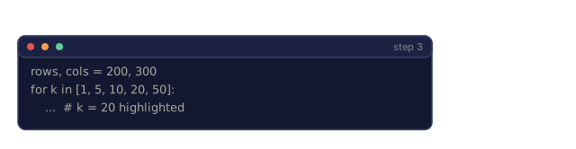
rows, cols = 200, 300
image = np.random.randn(rows, cols)

for k in [1, 5, 10, 20, 50]:
    compressed = compress_image_svd(image, k)
    error = np.linalg.norm(image - compressed) / np.linalg.norm(image)
    original_size = rows * cols
    compressed_size = k * (rows + cols + 1)
    ratio = compressed_size / original_size
    print(f"k={k:>3d}  error={error:.4f}  storage={ratio:.1%}")
Step 4: Noise reduction
np.random.seed(42)
clean = np.outer(np.sin(np.linspace(0, 4*np.pi, 100)),
                 np.cos(np.linspace(0, 2*np.pi, 80)))
noise = 0.3 * np.random.randn(100, 80)
noisy = clean + noise

U, S, Vt = np.linalg.svd(noisy, full_matrices=False)
denoised = U[:, :5] @ np.diag(S[:5]) @ Vt[:5, :]

print(f"Noisy error:    {np.linalg.norm(noisy - clean):.4f}")
print(f"Denoised error: {np.linalg.norm(denoised - clean):.4f}")
print(f"Improvement:    {(1 - np.linalg.norm(denoised - clean) / np.linalg.norm(noisy - clean)):.1%}")
Step 5: Pseudoinverse
A = np.array([[1, 1], [2, 1], [3, 1]], dtype=float)
b = np.array([3, 5, 6], dtype=float)

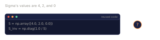
U, S, Vt = np.linalg.svd(A, full_matrices=False)
S_inv = np.diag(1.0 / S)
A_pinv = Vt.T @ S_inv @ U.T

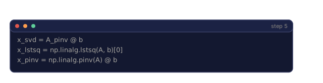
x_svd = A_pinv @ b
x_lstsq = np.linalg.lstsq(A, b, rcond=None)[0]
x_pinv = np.linalg.pinv(A) @ b

print(f"SVD pseudoinverse solution:  {x_svd}")
print(f"np.linalg.lstsq solution:   {x_lstsq}")
print(f"np.linalg.pinv solution:    {x_pinv}")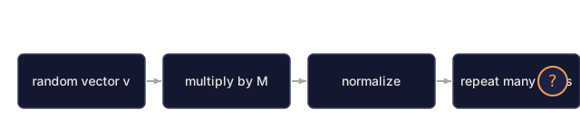
Use It
Full working demos live in code/svd.py. Run it and you'll see SVD applied back to back: image compression, recommendation systems, latent semantic analysis, noise reduction.
python svd.pyThe Julia version in code/svd.jl runs the same four demos through Julia's native svd() function and its LinearAlgebra package.
julia svd.jlShip It
This lesson produces:
outputs/skill-svd.md- a skill for knowing when to reach for SVD in a real project, and how to apply it once you do
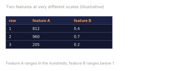
The numerical stability warning above isn't academic. The first time it cost me real debugging time, I'd computed PCA by hand: eigendecompose the covariance matrix, take the top eigenvectors, done. It worked fine until one feature happened to sit at a much smaller scale than the rest, and the components I got back were subtly off, not garbage, just wrong enough in the fourth decimal place to make a downstream model twitchy in a way that took a full afternoon to trace back to the PCA step. Switching to np.linalg.svd on the centered data directly fixed it immediately, because SVD never forms A^T A and never squares that condition number in the first place. If you only carry one operational habit out of this lesson, make it this: reach for SVD before you reach for eigendecomposition, even when they're mathematically equivalent on paper. On real data, they aren't equivalent in practice.
Exercises
-
Implement the full SVD from scratch without using power iteration. Instead, compute the eigendecomposition of A^T A to get V and the singular values, then compute U = A V Sigma^{-1}. Compare numerical accuracy with your power iteration version and with NumPy.
-
Load a real grayscale image (or convert one to grayscale). Compress it at ranks 1, 5, 10, 25, 50, 100. For each rank, compute the compression ratio and the relative error. Find the rank where the image becomes visually acceptable.
-
Build a tiny recommendation system. Create a 10x8 user-movie ratings matrix with some known entries. Fill missing entries with row means. Compute SVD and reconstruct a rank-3 approximation. Use the reconstructed matrix to predict the missing ratings. Verify that the predictions are reasonable.
-
Create a 100x50 document-term matrix with 3 synthetic topics. Each topic has 5 associated terms. Add noise. Apply SVD and verify that the top 3 singular values are much larger than the rest. Project documents into the 3D latent space and check that documents from the same topic cluster together.
-
Generate a clean low-rank matrix (rank 3, size 50x40) and add Gaussian noise at different levels (sigma = 0.1, 0.5, 1.0, 2.0). For each noise level, find the optimal truncation rank by sweeping k from 1 to 40 and measuring reconstruction error against the clean matrix. Plot how the optimal k changes with noise level.
Key Terms
| Term | What people say | What it actually means |
|---|---|---|
| SVD | "Factor any matrix" | Decompose A into U Sigma V^T where U and V are orthogonal and Sigma is diagonal with non-negative entries. Works for any matrix of any shape. |
| Singular value | "How important this component is" | The i-th diagonal entry of Sigma. Measures how much the matrix stretches along the i-th principal direction. Always non-negative, sorted in decreasing order. |
| Left singular vector | "Output direction" | A column of U. The direction in output space that the i-th right singular vector maps to (after scaling by sigma_i). |
| Right singular vector | "Input direction" | A column of V. The direction in input space that the matrix maps to the i-th left singular vector (after scaling by sigma_i). |
| Truncated SVD | "Low-rank approximation" | Keep only the top k singular values and their vectors. Produces the provably best rank-k approximation to the original matrix (Eckart-Young theorem). |
| Rank | "True dimensionality" | The number of non-zero singular values. Tells you how many independent directions the matrix actually uses. |
| Pseudoinverse | "Generalized inverse" | V Sigma+ U^T. Inverts non-zero singular values, leaves zeros as zeros. Solves least-squares problems for non-square or singular matrices. |
| Condition number | "How sensitive to errors" | sigma_max / sigma_min. A large condition number means small input changes cause large output changes. SVD reveals this directly. |
| Latent factor | "Hidden variable" | A dimension in the low-rank space discovered by SVD. In recommendations, a latent factor might correspond to genre preference. In NLP, it might correspond to a topic. |
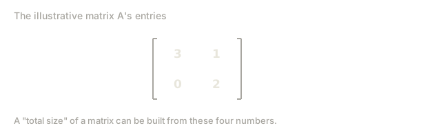
| Frobenius norm | "Total matrix size" | Square root of the sum of squared entries. Equals the square root of the sum of squared singular values. Used to measure approximation error. |
| Eckart-Young theorem | "SVD gives the best compression" | For any target rank k, the truncated SVD minimizes the approximation error over all possible rank-k matrices. |
| Power iteration | "Find the biggest eigenvector" | Repeatedly multiply a random vector by the matrix and normalize. Converges to the eigenvector with the largest eigenvalue. The building block of many SVD algorithms. |
Further Reading
- Gilbert Strang: Linear Algebra and Its Applications, Chapter 7 - thorough treatment of SVD with applications
- 3Blue1Brown: But what is the SVD? - geometric intuition for SVD
- We Recommend a Singular Value Decomposition - accessible overview from the American Mathematical Society
- Netflix Prize and Matrix Factorization - Simon Funk's original blog post on SVD for recommendations
- Latent Semantic Analysis - the original NLP application of SVD
- Numerical Linear Algebra by Trefethen and Bau - the gold standard for understanding SVD algorithms and their numerical properties