Matrix Transformations
A matrix isn't a grid of numbers sitting still. It's a set of instructions for reshaping space: rotate, stretch, tilt, flip. Learn what it does to one point and you know what it does to the whole plane.
Learning Objectives
- Construct rotation, scaling, shearing, and reflection matrices and apply them to 2D and 3D points
- Compose multiple transformations by matrix multiplication and verify that order matters
- Compute eigenvalues and eigenvectors of 2x2 matrices from the characteristic equation
- Explain why eigenvalues determine PCA directions, RNN stability, and spectral clustering behavior
The Problem
You read about PCA and see "find the eigenvectors of the covariance matrix." You read about model stability and see "check whether every eigenvalue has magnitude under 1." You read about data augmentation and see "apply a random rotation." None of that means anything until you can picture what a matrix actually does to space.
A matrix isn't a static grid of numbers. It's a machine: feed it a point, and it hands back a new point somewhere else in space. A rotation matrix spins points around the origin. A scaling matrix stretches or squashes them. A shearing matrix tilts them sideways. Every transformation a neural network applies to its data is one of these, or several of them stacked together. This lesson makes them concrete enough that the phrases above stop sounding like magic.


The Concept
Transformations as matrices
Every linear transformation in 2D reduces to a 2x2 matrix. That matrix tells you exactly where the basis vectors [1, 0] and [0, 1] land, and once you know that, everything else follows.

Rotation
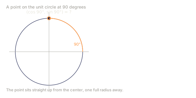
A 2D rotation by angle theta preserves distances and angles: every point just slides along a circular arc.

Analogy: picture a clock's hands sweeping around the pivot. Every point on the hand stays exactly as far from the center as it started, it just sweeps through an angle. A 2D rotation matrix does the same thing to every point in the plane at once, which is exactly what shows up in camera and robot pose estimation, 3D rendering, and rotation-based data augmentation for vision models.
In 3D, rotation happens around an axis, and each axis gets its own rotation matrix:
Rz(theta) = | cos  -sin  0 |     Rotate around z-axis
            | sin   cos  0 |     (x-y plane spins, z stays)
            |  0     0   1 |

Rx(theta) = | 1   0     0    |   Rotate around x-axis
            | 0  cos  -sin   |   (y-z plane spins, x stays)
            | 0  sin   cos   |

Ry(theta) = |  cos  0  sin |     Rotate around y-axis
            |   0   1   0  |     (x-z plane spins, y stays)
            | -sin  0  cos |
Scaling
Scaling stretches or compresses space along each axis, independently of the others.

Analogy: think of stretching a photo by different amounts along its width and height. Pull the horizontal handle and the image gets wider without getting taller; pull both and each direction stretches or squashes on its own. Feature normalization and the per-channel scaling inside batch norm both work exactly this way, one axis at a time.
Shearing
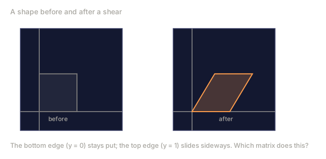
Shearing tilts one axis while the other stays fixed, turning rectangles into parallelograms.

Analogy: think of a deck of cards fanned out sideways on a table. Each card's top edge slides further than its bottom edge, so a neat stack of rectangles turns into a slanted stack of parallelograms. Image augmentation pipelines and perspective or deskew correction in document scanning both apply exactly this kind of tilt.
Shear matrices:
Shx = [[1, k], [0, 1]]shifts x by k * yShy = [[1, 0], [k, 1]]shifts y by k * x
Reflection
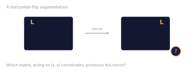
Reflection mirrors points across an axis or line, the way a mirror flips left and right.

Analogy: hold a page up to a mirror. The text is still the same size and shape, but it's flipped left to right. A reflection matrix does exactly that to every point in the plane at once, which is why horizontal-flip is one of the most common augmentations for vision models.
Reflection matrices:
- Reflect across y-axis:
[[-1, 0], [0, 1]] - Reflect across x-axis:
[[1, 0], [0, -1]]
Composition: chaining transformations
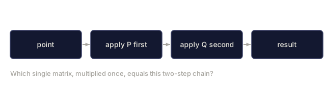
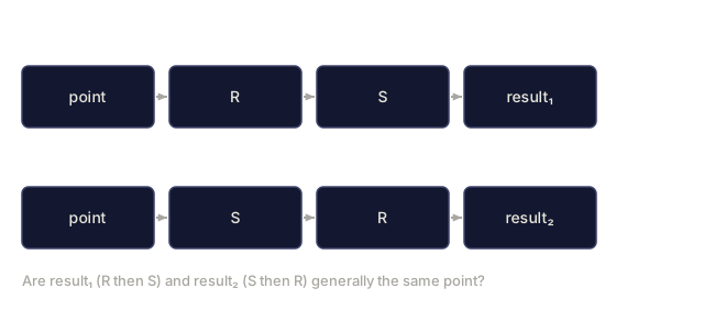
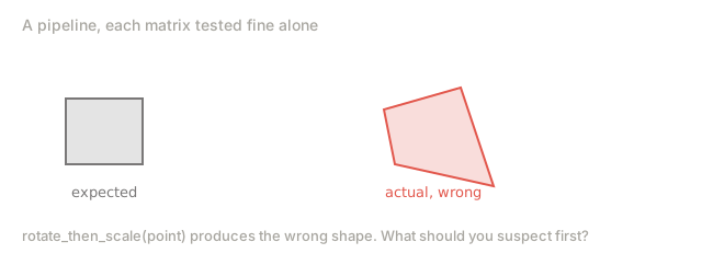
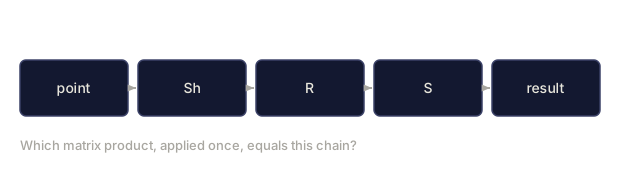
Chaining transformation A and then B is the same as multiplying their matrices: result = B @ A @ point. Order matters here, and it's easy to get backwards: rotating first and then scaling is not the same transformation as scaling first and then rotating.

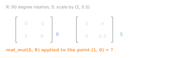
Composed: S @ R = [[0, -2], [0.5, 0]]

Composed: R @ S = [[0, -0.5], [2, 0]]
The results differ because matrix multiplication doesn't commute: S @ R and R @ S are, in general, two different matrices.
Analogy: think of two filters stacked on a camera lens. Light passes through the first, then the second. Swap the order and the final image changes, because the second filter now reacts to whatever the first one already did to the light, not to the original scene. Every multi-stage pipeline, from a robot's chain of coordinate-frame transforms to a stack of augmentations applied to one training image, has to get this order right.
Eigenvalues and eigenvectors
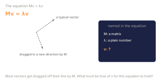
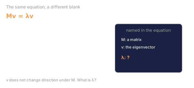
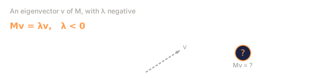
An eigenvector of a matrix is a direction the matrix only stretches or shrinks, never rotates: whatever comes out lies on the same line as the input, just longer, shorter, or flipped to the opposite direction if the eigenvalue is negative. That scale factor is the eigenvalue. Every other vector isn't so lucky; the matrix drags it off toward some new direction.
A @ v = lambda * v

v is the eigenvector (direction that survives)
lambda is the eigenvalue (how much it stretches)

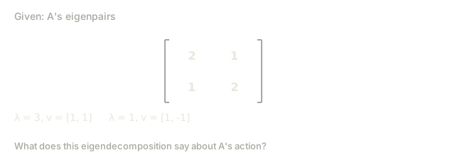
Example: A = | 2  1 |
             | 1  2 |

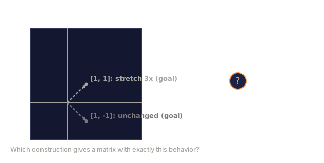
Eigenvector [1, 1] with eigenvalue 3:
  A @ [1,1] = [3, 3] = 3 * [1, 1]     (same direction, scaled by 3)

Eigenvector [1, -1] with eigenvalue 1:
  A @ [1,-1] = [1, -1] = 1 * [1, -1]  (same direction, unchanged)
This particular matrix stretches space 3x along [1, 1] and leaves [1, -1] exactly as it was. Every other direction is just some blend of those two.
Analogy: picture pulling on two opposite corners of a stretchy rubber sheet lying flat on a table. Most drawn lines on the sheet twist as it stretches, but the line running straight between the two corners you're pulling just gets longer along that same line. It never twists.
Eigendecomposition
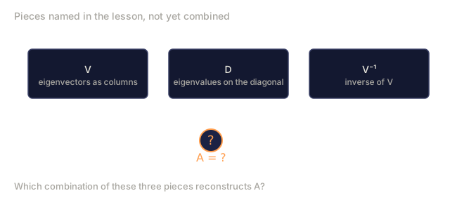
If a matrix has n linearly independent eigenvectors, you can decompose it entirely in terms of them:
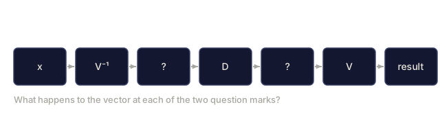
A = V @ D @ V^(-1)

V = matrix whose columns are eigenvectors
D = diagonal matrix of eigenvalues
V^(-1) = inverse of V

This says: change into eigenvector coordinates, scale along each axis, then change back.
Why eigenvalues matter
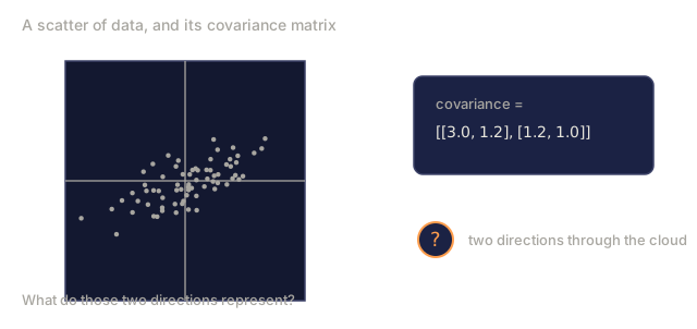
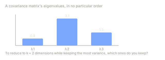
PCA. The eigenvectors of the covariance matrix are the principal components. The eigenvalues tell you how much variance each one captures. Sort by eigenvalue, keep the top k, and that's dimensionality reduction.
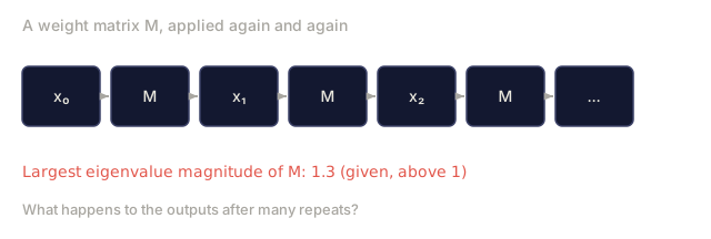
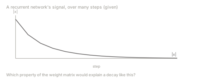
Stability. In recurrent networks and other dynamical systems, eigenvalues with magnitude greater than 1 make outputs explode over time. Magnitude less than 1 makes them vanish. That's the vanishing/exploding gradient problem, stated in one sentence.
Spectral methods. Graph neural networks use eigenvalues of the adjacency matrix. Spectral clustering uses eigenvalues of the Laplacian. Either way, the eigenvectors are what expose the graph's structure.
Determinant as volume scaling factor
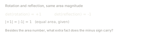
The determinant of a transformation matrix is a single number that tells you how much it scales area in 2D, or volume in 3D.
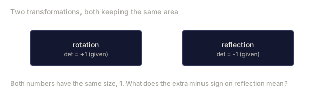
det = 1:   area preserved (rotation)
det = 2:   area doubled
det = 0:   space crushed to lower dimension (singular)
det = -1:  area preserved but orientation flipped (reflection)

| det(Rotation) | = 1        (always)
| det(Scale sx, sy) | = sx * sy
| det(Shear) | = 1           (area preserved)
det(Reflection) = -1        (orientation flipped)
Analogy: think of a recipe: double every ingredient and the dish comes out twice the size. That scaling factor is what the determinant measures for a matrix, applied to area or volume instead of a recipe. A negative determinant means the result also comes out mirror-flipped, not just resized. Checking whether a determinant (or, in normalizing flows, a Jacobian's determinant) is zero is exactly how you catch a transformation that has silently collapsed a dimension.









Build It
Step 1: Transformation matrices from scratch (Python)
import math

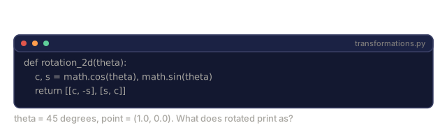
def rotation_2d(theta):
    c, s = math.cos(theta), math.sin(theta)
    return [[c, -s], [s, c]]

def scaling_2d(sx, sy):
    return [[sx, 0], [0, sy]]

def shearing_2d(kx, ky):
    return [[1, kx], [ky, 1]]

def reflection_x():
    return [[1, 0], [0, -1]]

def reflection_y():
    return [[-1, 0], [0, 1]]

def mat_vec_mul(matrix, vector):
    return [
        sum(matrix[i][j] * vector[j] for j in range(len(vector)))
        for i in range(len(matrix))
    ]

def mat_mul(a, b):
    rows_a, cols_b = len(a), len(b[0])
    cols_a = len(a[0])
    return [
        [sum(a[i][k] * b[k][j] for k in range(cols_a)) for j in range(cols_b)]
        for i in range(rows_a)
    ]

point = [1.0, 0.0]
angle = math.pi / 4

rotated = mat_vec_mul(rotation_2d(angle), point)
print(f"Rotate (1,0) by 45 deg: ({rotated[0]:.4f}, {rotated[1]:.4f})")

scaled = mat_vec_mul(scaling_2d(2, 3), [1.0, 1.0])
print(f"Scale (1,1) by (2,3): ({scaled[0]:.1f}, {scaled[1]:.1f})")

sheared = mat_vec_mul(shearing_2d(1, 0), [1.0, 1.0])
print(f"Shear (1,1) kx=1: ({sheared[0]:.1f}, {sheared[1]:.1f})")

reflected = mat_vec_mul(reflection_y(), [2.0, 1.0])
print(f"Reflect (2,1) across y: ({reflected[0]:.1f}, {reflected[1]:.1f})")
Step 2: Composition of transformations
R = rotation_2d(math.pi / 2)
S = scaling_2d(2, 0.5)

rotate_then_scale = mat_mul(S, R)
scale_then_rotate = mat_mul(R, S)

point = [1.0, 0.0]
result1 = mat_vec_mul(rotate_then_scale, point)
result2 = mat_vec_mul(scale_then_rotate, point)

print(f"Rotate 90 then scale: ({result1[0]:.2f}, {result1[1]:.2f})")
print(f"Scale then rotate 90: ({result2[0]:.2f}, {result2[1]:.2f})")
print(f"Same? {result1 == result2}")
Step 3: Eigenvalues from scratch (2x2)
A 2x2 matrix [[a, b], [c, d]] has eigenvalues that solve the characteristic equation: lambda^2 - (a+d)*lambda + (ad - bc) = 0.
def eigenvalues_2x2(matrix):
    a, b = matrix[0]
    c, d = matrix[1]
    trace = a + d
    det = a * d - b * c
    discriminant = trace ** 2 - 4 * det
    if discriminant < 0:
        real = trace / 2
        imag = (-discriminant) ** 0.5 / 2
        return (complex(real, imag), complex(real, -imag))
    sqrt_disc = discriminant ** 0.5
    return ((trace + sqrt_disc) / 2, (trace - sqrt_disc) / 2)

def eigenvector_2x2(matrix, eigenvalue):
    a, b = matrix[0]
    c, d = matrix[1]
    if abs(b) > 1e-10:
        v = [b, eigenvalue - a]
    elif abs(c) > 1e-10:
        v = [eigenvalue - d, c]
    else:
        if abs(a - eigenvalue) < 1e-10:
            v = [1, 0]
        else:
            v = [0, 1]
    mag = (v[0] ** 2 + v[1] ** 2) ** 0.5
    return [v[0] / mag, v[1] / mag]

A = [[2, 1], [1, 2]]
vals = eigenvalues_2x2(A)
print(f"Matrix: {A}")
print(f"Eigenvalues: {vals[0]:.4f}, {vals[1]:.4f}")

for val in vals:
    vec = eigenvector_2x2(A, val)
    result = mat_vec_mul(A, vec)
    scaled = [val * vec[0], val * vec[1]]
    print(f"  lambda={val:.1f}, v={[round(x,4) for x in vec]}")
    print(f"    A@v = {[round(x,4) for x in result]}")
    print(f"    l*v = {[round(x,4) for x in scaled]}")
Step 4: Determinant as volume scaling factor
def det_2x2(matrix):
    return matrix[0][0] * matrix[1][1] - matrix[0][1] * matrix[1][0]

print(f"det(rotation 45) = {det_2x2(rotation_2d(math.pi/4)):.4f}")
print(f"det(scale 2,3)   = {det_2x2(scaling_2d(2, 3)):.1f}")
print(f"det(shear kx=1)  = {det_2x2(shearing_2d(1, 0)):.1f}")
print(f"det(reflect y)   = {det_2x2(reflection_y()):.1f}")

singular = [[1, 2], [2, 4]]
print(f"det(singular)     = {det_2x2(singular):.1f}")
print("Singular: columns are proportional, space collapses to a line.")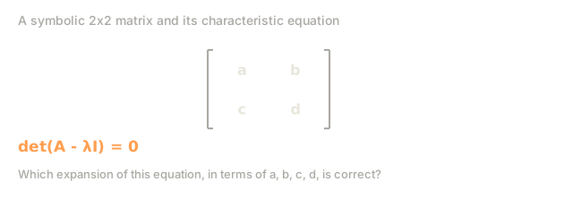



Use It
NumPy already does all of this, faster than any of the loops above, and it's what you'll actually reach for.
import numpy as np

theta = np.pi / 4
R = np.array([[np.cos(theta), -np.sin(theta)],
              [np.sin(theta),  np.cos(theta)]])

point = np.array([1.0, 0.0])
print(f"Rotate (1,0) by 45 deg: {R @ point}")

S = np.diag([2.0, 3.0])
composed = S @ R
print(f"Scale(2,3) after Rotate(45): {composed @ point}")

A = np.array([[2, 1], [1, 2]], dtype=float)
eigenvalues, eigenvectors = np.linalg.eig(A)
print(f"\nEigenvalues: {eigenvalues}")
print(f"Eigenvectors (columns):\n{eigenvectors}")

for i in range(len(eigenvalues)):
    v = eigenvectors[:, i]
    lam = eigenvalues[i]
    print(f"  A @ v{i} = {A @ v}, lambda * v{i} = {lam * v}")

print(f"\ndet(R) = {np.linalg.det(R):.4f}")
print(f"det(S) = {np.linalg.det(S):.1f}")

B = np.array([[3, 1], [0, 2]], dtype=float)
vals, vecs = np.linalg.eig(B)
D = np.diag(vals)
V = vecs
reconstructed = V @ D @ np.linalg.inv(V)
print(f"\nEigendecomposition A = V @ D @ V^-1:")
print(f"Original:\n{B}")
print(f"Reconstructed:\n{reconstructed}")
3D rotations with NumPy
def rotation_3d_z(theta):
    c, s = np.cos(theta), np.sin(theta)
    return np.array([[c, -s, 0], [s, c, 0], [0, 0, 1]])

def rotation_3d_x(theta):
    c, s = np.cos(theta), np.sin(theta)
    return np.array([[1, 0, 0], [0, c, -s], [0, s, c]])

point_3d = np.array([1.0, 0.0, 0.0])
rotated_z = rotation_3d_z(np.pi / 2) @ point_3d
rotated_x = rotation_3d_x(np.pi / 2) @ point_3d

print(f"\n3D point: {point_3d}")
print(f"Rotate 90 around z: {np.round(rotated_z, 4)}")
print(f"Rotate 90 around x: {np.round(rotated_x, 4)}")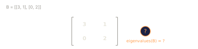

Ship It
This lesson lays the geometric groundwork for PCA (Phase 2) and for reading what a neural network's weights actually do to its inputs. The eigenvalue and eigenvector code you just built isn't a simplified stand-in for the real thing: it's the same algorithm running underneath dimensionality reduction, spectral clustering, and stability analysis in production systems.
The bug I've seen bite more people here than any other is composition order. You write rotate(scale(point)), feel good about it, and then wonder why the picture doesn't match what you expected. Function composition and matrix composition read in the same direction, right to left, innermost first, but it is easy to flip that around in your head the first dozen times you do it. When a transformed shape looks wrong, don't start by second-guessing the matrix entries. Print the point after each individual transform, one step at a time, and compare each step against what that single operation should do on its own. Nearly every "my eigendecomposition is broken" bug I've actually chased down turned out to be a composition-order mistake two steps earlier, not a problem with the eigenvectors at all.
Exercises
-
Apply rotation, scaling, and shearing to a unit square (corners at [0,0], [1,0], [1,1], [0,1]). Print the transformed corners for each. Verify that rotation preserves distances between corners.
-
Find the eigenvalues of the matrix [[4, 2], [1, 3]] by hand using the characteristic equation. Then verify with your from-scratch function and with NumPy.
-
Create a composition of three transformations (rotate 30 degrees, scale by [1.5, 0.8], shear with kx=0.3) and apply it to 8 points arranged in a circle. Print before and after coordinates. Compute the determinant of the composed matrix and verify it equals the product of the individual determinants.
Key Terms
| Term | What people say | What it actually means |
|---|---|---|
| Rotation matrix | "Spins things" | An orthogonal matrix that moves points along circular arcs while preserving distances and angles. Determinant is always 1. |
| Scaling matrix | "Makes things bigger" | A diagonal matrix that stretches or compresses independently along each axis. Determinant is the product of scale factors. |
| Shearing matrix | "Slants things" | A matrix that shifts one coordinate proportionally to another, turning rectangles into parallelograms. Determinant is 1. |
| Reflection | "Mirrors things" | A matrix that flips space across an axis or plane. Determinant is -1. |
| Composition | "Do two things" | Multiplying transformation matrices to chain operations. Order matters: B @ A means apply A first, then B. |
| Eigenvector | "Special direction" | A direction that the matrix only scales, never rotates. The transformation's fingerprint. |
| Eigenvalue | "How much it stretches" | The scalar factor by which the matrix scales its eigenvector. Can be negative (flip) or complex (rotation). |
| Eigendecomposition | "Break the matrix apart" | Writing a matrix as V @ D @ V^(-1), separating it into its fundamental scaling directions and magnitudes. |
| Determinant | "A single number from a matrix" | The factor by which the transformation scales area (2D) or volume (3D). Zero means the transformation is irreversible. |
| Characteristic equation | "Where eigenvalues come from" | det(A - lambda * I) = 0. The polynomial whose roots are the eigenvalues. |
Further Reading
- 3Blue1Brown: Linear Transformations -- visual intuition for how matrices reshape space
- 3Blue1Brown: Eigenvectors and Eigenvalues -- the best visual explanation of what eigenvectors mean geometrically
- MIT 18.06 Lecture 21: Eigenvalues and Eigenvectors -- Gilbert Strang's classic treatment
Code
- transformations.jl (text, 252 lines)
- transformations.py (python, 355 lines)