Calculus for Machine Learning
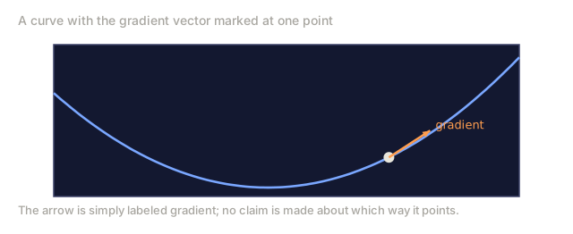
A derivative tells you which way is downhill. That's the entire trick a neural network uses to learn.
Learning Objectives
- Compute numerical and analytical derivatives for common ML functions (x^2, sigmoid, cross-entropy)
- Implement gradient descent from scratch to minimize a loss function in 1D and 2D
- Derive the gradient of a linear regression model and train it via manual weight updates
- Explain the Hessian matrix, Taylor series approximations, and their connection to optimization methods
The Problem
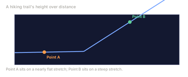
A neural network can have millions of weights, and every one of them is a knob. Training means turning each knob in whatever direction makes the model slightly less wrong. Calculus is what tells you that direction.
Without it, you'd be trying random changes and hoping for the best. With a derivative for every weight, you know exactly how nudging that one number moves the error, so you turn each knob the right way instead of guessing.
The Concept
What is a derivative?
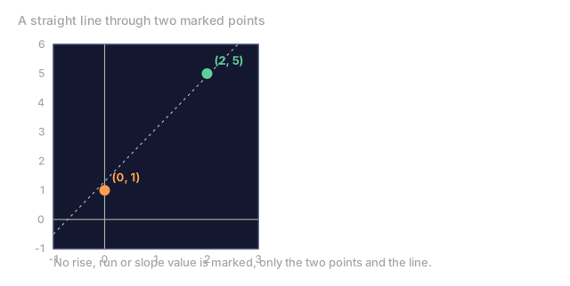
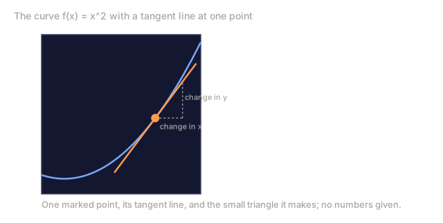
A derivative measures the rate of change: for a function y = f(x), f'(x) tells you how much y moves when you nudge x by a tiny amount.
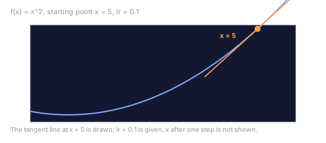
Geometrically, it's the slope of the tangent line at that point.
f(x) = x^2:
| x | f(x) | f'(x) (slope) |
|---|---|---|
| 0 | 0 | 0 (flat, at the bottom) |
| 1 | 1 | 2 |
| 2 | 4 | 4 (tangent line slope at this point) |
| 3 | 9 | 6 |
At x=2 the slope is 4: nudge x slightly to the right and y moves by roughly four times that nudge. At x=0 the slope is 0, so you're sitting at the bottom of the bowl.
The formal definition:
f'(x) = lim   f(x + h) - f(x)
        h->0  -----------------
                     h
In code, skip the limit and use a very small h instead. That's the numerical derivative.
Partial derivatives: one variable at a time
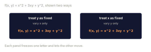
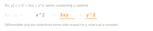
A partial derivative holds every variable constant except one, then takes the derivative with respect to that single variable. Real functions have many inputs, and a neural network's loss depends on thousands of weights, so isolating the effect of just one of them at a time is exactly what a partial derivative gives you.
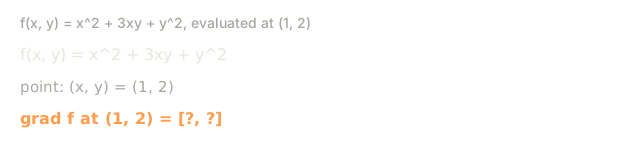
f(x, y) = x^2 + 3xy + y^2

df/dx = 2x + 3y     (treat y as a constant)
df/dy = 3x + 2y     (treat x as a constant)
Each partial derivative answers one question: nudge just this one weight, how does the loss move?
The gradient: vector of all partial derivatives
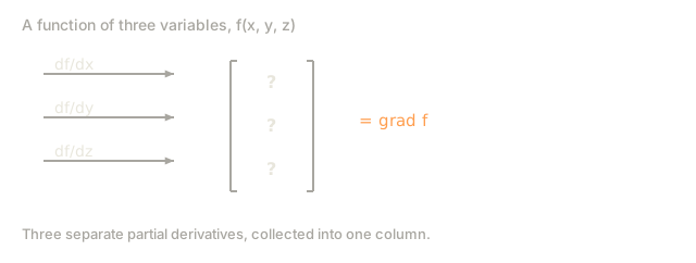
The gradient collects every partial derivative into a single vector. For a function f(x, y, z):
grad f = [ df/dx, df/dy, df/dz ]
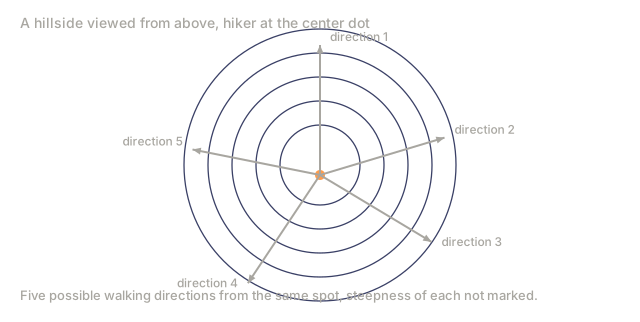
It points in the direction of steepest ascent, so to minimize a function you walk the opposite way.
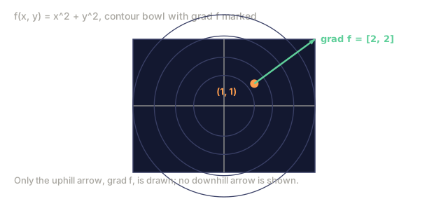
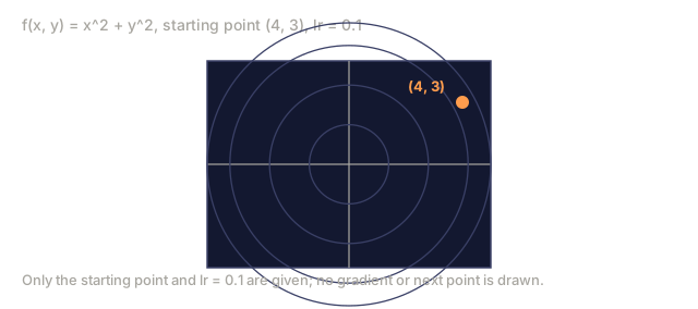
Contour plot of f(x,y) = x^2 + y^2:
The function forms a bowl shape with concentric circles as contour lines. The minimum is at (0, 0).
| Point | grad f | -grad f (descent direction) |
|---|---|---|
| (1, 1) | [2, 2] (points uphill, away from minimum) | [-2, -2] (points downhill, toward minimum) |
| (0, 0) | [0, 0] (flat, at the minimum) | [0, 0] |
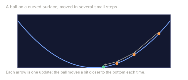
That's gradient descent in one picture: compute the gradient, flip its sign, take a step.
The connection to optimization
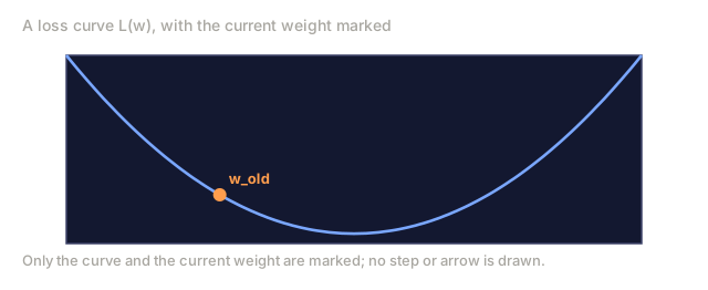
Training a neural network is an optimization problem. The loss function L(w1, w2, ..., wn) measures how wrong the model is, and the goal is to minimize it.
Gradient descent update rule:

  w_new = w_old - learning_rate * dL/dw

For every weight:
  1. Compute the partial derivative of loss with respect to that weight
  2. Subtract a small multiple of it from the weight
  3. Repeat
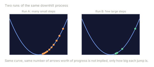
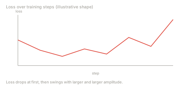
The learning rate sets the step size: too big and you overshoot the minimum, too small and you crawl toward it.
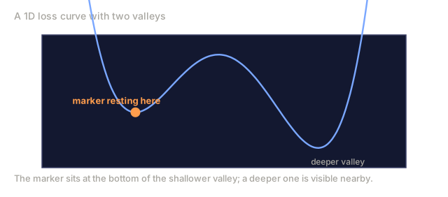
Loss landscape (1D slice):
The loss function L(w) forms a curve with peaks and valleys as the weight w varies.
| Feature | Description |
|---|---|
| Global minimum | The lowest point on the entire curve: the best solution |
| Local minimum | A valley that is lower than its neighbors but not the lowest overall |
| Slope | Gradient descent follows the slope downhill from any starting point |
Gradient descent just follows the slope downhill. It can get stuck in a local minimum, but in a high-dimensional space with millions of weights, that turns out to rarely matter in practice.
Numerical vs analytical derivatives
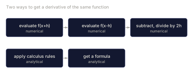
There are two ways to compute a derivative.
Analytical: apply the rules of calculus by hand. For f(x) = x^2, that gives f'(x) = 2x. Exact. Fast.
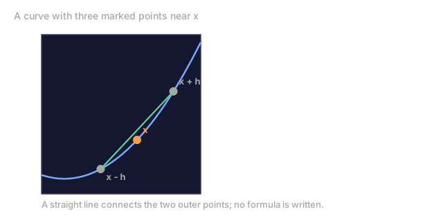
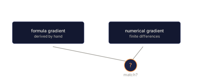
Numerical: approximate straight from the definition. Compute f(x+h) and f(x-h) for a tiny h, then take the difference.
Numerical (central difference):

f'(x) ~= f(x + h) - f(x - h)
          -----------------------
                  2h

h = 0.0001 works well in practice
Numerical derivatives are slower but work for any function; analytical derivatives are fast but require deriving the formula by hand. Neural network frameworks use a third approach: automatic differentiation, which computes exact derivatives mechanically. You'll meet it in Phase 3.
Derivatives by hand for simple functions
You'll see these same derivatives over and over in ML.
Function        Derivative       Used in
--------        ----------       -------
f(x) = x^2     f'(x) = 2x      Loss functions (MSE)
f(x) = wx + b  f'(w) = x        Linear layer (gradient w.r.t. weight)
                f'(b) = 1        Linear layer (gradient w.r.t. bias)
                f'(x) = w        Linear layer (gradient w.r.t. input)
f(x) = e^x     f'(x) = e^x     Softmax, attention
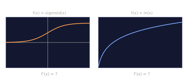
f(x) = ln(x)   f'(x) = 1/x     Cross-entropy loss
f(x) = 1/(1+e^-x)  f'(x) = f(x)(1-f(x))   Sigmoid activation
For f(x) = x^2:
f(x) = x^2    f'(x) = 2x

  x    f(x)   f'(x)   meaning
  -2    4      -4      slope tilts left (decreasing)
  -1    1      -2      slope tilts left (decreasing)
   0    0       0      flat (minimum!)
   1    1       2      slope tilts right (increasing)
   2    4       4      slope tilts right (increasing)
For f(w) = wx + b with x=3, b=1:
f(w) = 3w + 1    f'(w) = 3

The derivative with respect to w is just x.
If x is big, a small change in w causes a big change in output.
The chain rule
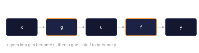
The chain rule tells you how to differentiate a composition of functions.
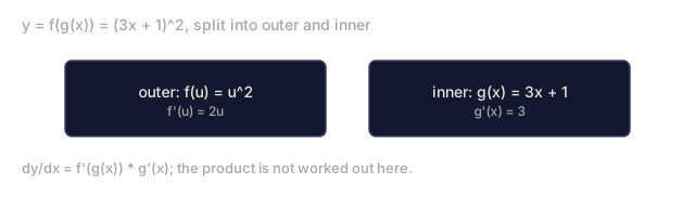
If y = f(g(x)), then dy/dx = f'(g(x)) * g'(x)

Example: y = (3x + 1)^2
  outer: f(u) = u^2       f'(u) = 2u
  inner: g(x) = 3x + 1    g'(x) = 3
  dy/dx = 2(3x + 1) * 3 = 6(3x + 1)
A neural network is nothing but a chain of functions: input -> linear -> activation -> linear -> activation -> loss. Backpropagation is the chain rule applied over and over, from output back to input. That's the entire algorithm.
The Hessian Matrix
The gradient tells you the slope. The Hessian tells you the curvature.
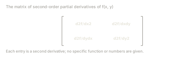
The Hessian is the matrix of second-order partial derivatives. For a function f(x1, x2, ..., xn), entry (i, j) of the Hessian is:
H[i][j] = d^2f / (dx_i * dx_j)
For a 2-variable function f(x, y):
H = | d^2f/dx^2    d^2f/dxdy |
    | d^2f/dydx    d^2f/dy^2 |
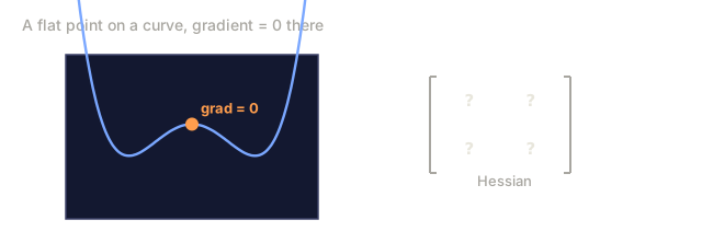
What the Hessian tells you at a critical point (where gradient = 0):
| Hessian property | Meaning | Example surface |
|---|---|---|
| Positive definite (all eigenvalues > 0) | Local minimum | Bowl pointing up |
| Negative definite (all eigenvalues < 0) | Local maximum | Bowl pointing down |
| Indefinite (mixed eigenvalues) | Saddle point | Horse saddle shape |
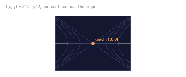
Example: f(x, y) = x^2 - y^2 (a saddle function)
df/dx = 2x       df/dy = -2y
d^2f/dx^2 = 2    d^2f/dy^2 = -2    d^2f/dxdy = 0

H = | 2   0 |
    | 0  -2 |

Eigenvalues: 2 and -2 (one positive, one negative)
--> Saddle point at (0, 0)
Compare with f(x, y) = x^2 + y^2 (a bowl):
H = | 2  0 |
    | 0  2 |

Eigenvalues: 2 and 2 (both positive)
--> Local minimum at (0, 0)
Why the Hessian matters in ML:
Newton's method uses the Hessian to take better optimization steps than gradient descent. Instead of just following the slope, it accounts for curvature:
Newton's update:    w_new = w_old - H^(-1) * gradient
Gradient descent:   w_new = w_old - lr * gradient
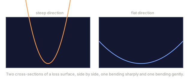
Newton's method converges faster because the Hessian "rescales" the gradient: steep directions get smaller steps, flat directions get larger steps.
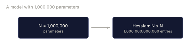
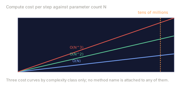
The catch: for a neural network with N parameters, the Hessian is N x N. A model with 1 million parameters would need a 1 trillion-entry matrix, which is why practical optimizers approximate it instead of computing it directly.
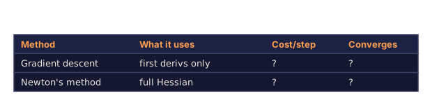
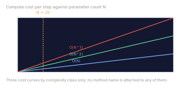
| Method | What it uses | Cost | Convergence |
|---|---|---|---|
| Gradient descent | First derivatives only | O(N) per step | Slow (linear) |
| Newton's method | Full Hessian | O(N^3) per step | Fast (quadratic) |
| L-BFGS | Approximate Hessian from gradient history | O(N) per step | Medium (superlinear) |
| Adam | Per-parameter adaptive rates (diagonal Hessian approx) | O(N) per step | Medium |
| Natural gradient | Fisher information matrix (statistical Hessian) | O(N^2) per step | Fast |
In practice, Adam is the default optimizer in deep learning: it approximates second-order information cheaply by tracking a running mean and variance of the gradients for each parameter.
Taylor Series Approximation
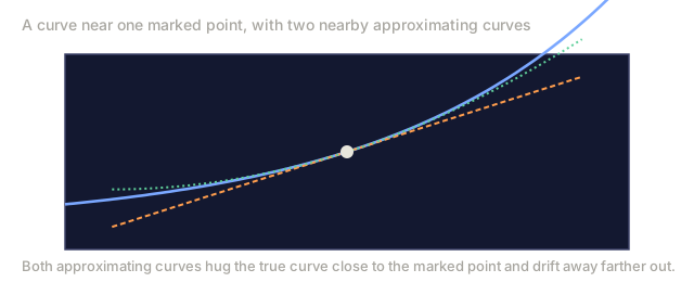
Any smooth function can be approximated locally by a polynomial:
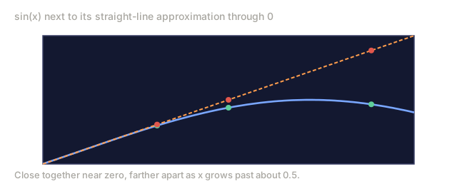
f(x + h) = f(x) + f'(x)*h + (1/2)*f''(x)*h^2 + (1/6)*f'''(x)*h^3 + ...
The more terms you include, the better the approximation gets, though only close to x.
Why Taylor series matter for ML:
-
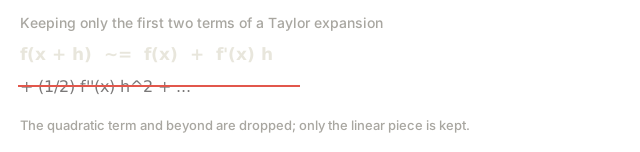
First-order Taylor = gradient descent. When you use f(x + h) ~ f(x) + f'(x)*h, you are making a linear approximation. Gradient descent minimizes this linear model to choose h = -lr * f'(x).
-
Second-order Taylor = Newton's method. Using f(x + h) ~ f(x) + f'(x)*h + (1/2)*f''(x)*h^2, you get a quadratic model. Minimizing it gives h = -f'(x)/f''(x), which is exactly Newton's step.
-
Loss function design. MSE and cross-entropy are smooth, which means their Taylor expansions are well-behaved. This is not an accident. Smooth losses make optimization predictable.
Approximation order    What it captures    Optimization method
-------------------    -----------------   -------------------
0th order (constant)   Just the value      Random search
1st order (linear)     Slope               Gradient descent
2nd order (quadratic)  Curvature           Newton's method
Higher orders          Finer structure     Rarely used in ML
The key insight: every gradient-based optimizer is doing the same thing, approximating the loss function locally and stepping to the minimum of that approximation.
Integrals in ML
Derivatives tell you rates of change. Integrals compute accumulation: area under a curve.
In ML, you rarely compute integrals by hand, but the concept is everywhere:
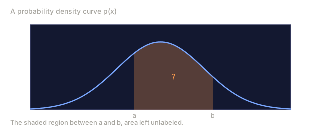
Probability. For a continuous random variable with density p(x):
P(a < X < b) = integral from a to b of p(x) dx
The area under the probability density curve between a and b is the probability of landing in that range.
Expected value. The average outcome weighted by probability:
E[f(X)] = integral of f(x) * p(x) dx
The expected loss over a data distribution is an integral. Training minimizes an empirical approximation of this.
KL divergence. Measures how different two distributions are:
KL(p || q) = integral of p(x) * log(p(x) / q(x)) dx
Used in VAEs, knowledge distillation, and Bayesian inference.
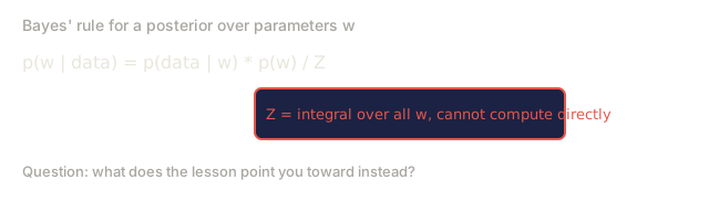
Normalization constants. In Bayesian inference:
p(w | data) = p(data | w) * p(w) / integral of p(data | w) * p(w) dw
The denominator is an integral over all possible parameter values. It is often intractable, which is why we use approximations like MCMC and variational inference.
| Integral concept | Where it appears in ML |
|---|---|
| Area under curve | Probability from density functions |
| Expected value | Loss functions, risk minimization |
| KL divergence | VAEs, policy optimization, distillation |
| Normalization | Bayesian posteriors, softmax denominator |
| Marginal likelihood | Model comparison, evidence lower bound (ELBO) |
Multivariable Chain Rule in a Computation Graph
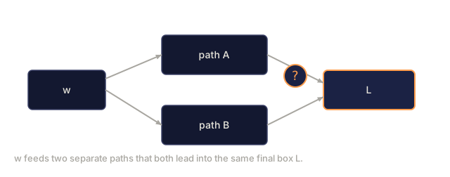
The chain rule isn't limited to a straight line of scalar functions. In a neural network, variables fan out and merge, and here's how derivatives flow through a simple forward pass:

The backward pass runs the same graph right to left, computing gradients:

Each arrow multiplies by its local derivative, and the gradient for any parameter is the product of every local derivative along the path from loss back to that parameter. Where paths branch and merge, you sum the contributions: that's the multivariate chain rule.
That's the whole of backpropagation: the chain rule applied mechanically across a computation graph, from output back to every input.
The Jacobian matrix
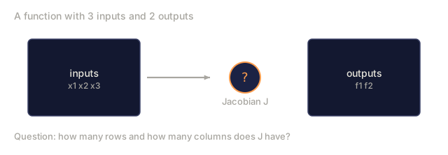
The Jacobian is the matrix containing every partial derivative of every output with respect to every input. Whenever a function maps a vector to a vector, the way a neural network layer does, that's the shape its derivative takes.
For f: R^n -> R^m, the Jacobian J is an m x n matrix:
| x1 | x2 | ... | xn | |
|---|---|---|---|---|
| f1 | df1/dx1 | df1/dx2 | ... | df1/dxn |
| f2 | df2/dx1 | df2/dx2 | ... | df2/dxn |
| ... | ... | ... | ... | ... |
| fm | dfm/dx1 | dfm/dx2 | ... | dfm/dxn |
You'll never compute a Jacobian by hand for a real network; PyTorch handles that. But knowing it exists tells you what to expect from the shapes in backpropagation: a layer that maps R^n to R^m has an m x n Jacobian, and the gradient flows backward through its transpose.
Why this matters for neural networks
Every weight in a neural network gets its own gradient, and that gradient tells you exactly how to nudge the weight to shrink the loss.


Each weight update:
W1 = W1 - lr * dL/dW1W2 = W2 - lr * dL/dW2
The forward pass produces a prediction and a loss. The backward pass turns that loss into a gradient for every weight. Every weight takes a small step downhill, and you repeat that millions of times. That's deep learning.


Build It
Step 1: Numerical derivative from scratch
def numerical_derivative(f, x, h=1e-7):
    return (f(x + h) - f(x - h)) / (2 * h)

def f(x):
    return x ** 2

for x in [-2, -1, 0, 1, 2]:
    numerical = numerical_derivative(f, x)
    analytical = 2 * x
    print(f"x={x:2d}  f'(x) numerical={numerical:.6f}  analytical={analytical:.1f}")
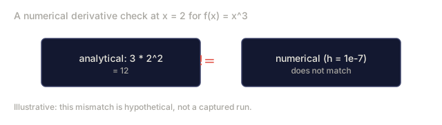
The numerical result matches the analytical one out to many decimal places.
Step 2: Partial derivatives and gradients
def numerical_gradient(f, point, h=1e-7):
    gradient = []
    for i in range(len(point)):
        point_plus = list(point)
        point_minus = list(point)
        point_plus[i] += h
        point_minus[i] -= h
        partial = (f(point_plus) - f(point_minus)) / (2 * h)
        gradient.append(partial)
    return gradient

def f_multi(point):
    x, y = point
    return x**2 + 3*x*y + y**2

grad = numerical_gradient(f_multi, [1.0, 2.0])
print(f"Numerical gradient at (1,2): {[f'{g:.4f}' for g in grad]}")
print(f"Analytical gradient at (1,2): [2*1+3*2, 3*1+2*2] = [{2*1+3*2}, {3*1+2*2}]")
Step 3: Gradient descent to find the minimum of f(x) = x^2
x = 5.0
lr = 0.1
for step in range(20):
    grad = 2 * x
    x = x - lr * grad
    print(f"step {step:2d}  x={x:8.4f}  f(x)={x**2:10.6f}")
Starting from x=5, each step lands closer to the minimum at x=0.
Step 4: Gradient descent on a 2D function
def f_2d(point):
    x, y = point
    return x**2 + y**2

point = [4.0, 3.0]
lr = 0.1
for step in range(30):
    grad = numerical_gradient(f_2d, point)
    point = [p - lr * g for p, g in zip(point, grad)]
    loss = f_2d(point)
    if step % 5 == 0 or step == 29:
        print(f"step {step:2d}  point=({point[0]:7.4f}, {point[1]:7.4f})  f={loss:.6f}")
Step 5: Comparing numerical and analytical derivatives
import math

test_functions = [
    ("x^2",      lambda x: x**2,          lambda x: 2*x),
    ("x^3",      lambda x: x**3,          lambda x: 3*x**2),
    ("sin(x)",   lambda x: math.sin(x),   lambda x: math.cos(x)),
    ("e^x",      lambda x: math.exp(x),   lambda x: math.exp(x)),
    ("1/x",      lambda x: 1/x,           lambda x: -1/x**2),
]

x = 2.0
print(f"{'Function':<12} {'Numerical':>12} {'Analytical':>12} {'Error':>12}")
print("-" * 50)
for name, f, df in test_functions:
    num = numerical_derivative(f, x)
    ana = df(x)
    err = abs(num - ana)
    print(f"{name:<12} {num:12.6f} {ana:12.6f} {err:12.2e}")
Step 6: Computing the Hessian numerically
def hessian_2d(f, x, y, h=1e-5):
    fxx = (f(x + h, y) - 2 * f(x, y) + f(x - h, y)) / (h ** 2)
    fyy = (f(x, y + h) - 2 * f(x, y) + f(x, y - h)) / (h ** 2)
    fxy = (f(x + h, y + h) - f(x + h, y - h) - f(x - h, y + h) + f(x - h, y - h)) / (4 * h ** 2)
    return [[fxx, fxy], [fxy, fyy]]

def saddle(x, y):
    return x ** 2 - y ** 2

def bowl(x, y):
    return x ** 2 + y ** 2

H_saddle = hessian_2d(saddle, 0.0, 0.0)
H_bowl = hessian_2d(bowl, 0.0, 0.0)
print(f"Saddle Hessian: {H_saddle}")  # [[2, 0], [0, -2]] -- mixed signs
print(f"Bowl Hessian:   {H_bowl}")    # [[2, 0], [0, 2]]  -- both positive
The saddle's Hessian has eigenvalues 2 and -2, mixed signs, confirming a saddle point. The bowl's Hessian has eigenvalues 2 and 2, both positive, confirming a minimum.
Step 7: Taylor approximation in action
import math

def taylor_approx(f, f_prime, f_double_prime, x0, h, order=2):
    result = f(x0)
    if order >= 1:
        result += f_prime(x0) * h
    if order >= 2:
        result += 0.5 * f_double_prime(x0) * h ** 2
    return result

x0 = 0.0
for h in [0.1, 0.5, 1.0, 2.0]:
    true_val = math.sin(h)
    t1 = taylor_approx(math.sin, math.cos, lambda x: -math.sin(x), x0, h, order=1)
    t2 = taylor_approx(math.sin, math.cos, lambda x: -math.sin(x), x0, h, order=2)
    print(f"h={h:.1f}  sin(h)={true_val:.4f}  order1={t1:.4f}  order2={t2:.4f}")
Near x0=0, sin(x) ~ x is the first-order Taylor approximation. It's excellent for small h and breaks down for large h, which is why gradient descent works best with small learning rates: each step assumes the linear approximation is accurate.
Step 8: Why this matters for a neural network
import random

random.seed(42)

w = random.gauss(0, 1)
b = random.gauss(0, 1)
lr = 0.01

xs = [1.0, 2.0, 3.0, 4.0, 5.0]
ys = [3.0, 5.0, 7.0, 9.0, 11.0]

for epoch in range(200):
    total_loss = 0
    dw = 0
    db = 0
    for x, y in zip(xs, ys):
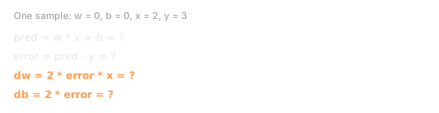
        pred = w * x + b
        error = pred - y
        total_loss += error ** 2
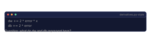
        dw += 2 * error * x
        db += 2 * error
    dw /= len(xs)
    db /= len(xs)
    total_loss /= len(xs)
    w -= lr * dw
    b -= lr * db
    if epoch % 40 == 0 or epoch == 199:
        print(f"epoch {epoch:3d}  w={w:.4f}  b={b:.4f}  loss={total_loss:.6f}")

print(f"\nLearned: y = {w:.2f}x + {b:.2f}")
print(f"Actual:  y = 2x + 1")
Every gradient-based training loop follows exactly this pattern: predict, compute the loss, compute the gradients, update the weights.

Use It
NumPy gives you the same operations, just faster and more concise:
import numpy as np

x = np.array([1, 2, 3, 4, 5], dtype=float)
y = np.array([3, 5, 7, 9, 11], dtype=float)

w, b = np.random.randn(), np.random.randn()
lr = 0.01

for epoch in range(200):
    pred = w * x + b
    error = pred - y
    loss = np.mean(error ** 2)
    dw = np.mean(2 * error * x)
    db = np.mean(2 * error)
    w -= lr * dw
    b -= lr * db

print(f"Learned: y = {w:.2f}x + {b:.2f}")
You just built gradient descent from scratch by hand. PyTorch will automate the gradient computation later, but the update loop underneath is identical.
The first time I trained a model without understanding what backward() was actually doing, I spent two days chasing a bug that turned out to be a completely correct gradient — I just didn't believe the number because I couldn't have predicted it myself. Once you've computed a handful of these derivatives by hand and watched gradient descent take its first few steps, autodiff stops being a black box and becomes what it actually is: a shortcut. It's faster than working out the chain rule by hand every time, not a replacement for knowing what the chain rule is doing. Build the numerical gradient checker from Build It before you trust anyone else's autograd, PyTorch included.
Exercises
- Implement
numerical_second_derivative(f, x)usingnumerical_derivativecalled twice. Verify that the second derivative of x^3 at x=2 is 12. - Use gradient descent to find the minimum of f(x, y) = (x - 3)^2 + (y + 1)^2. Start from (0, 0). The answer should converge to (3, -1).
- Add momentum to the gradient descent loop: maintain a velocity vector that accumulates past gradients. Compare convergence speed with and without momentum on f(x) = x^4 - 3x^2.
Key Terms
| Term | What people say | What it actually means |
|---|---|---|
| Derivative | "The slope" | The rate of change of a function at a point. Tells you how much the output changes per unit change in input. |
| Partial derivative | "Derivative of one variable" | The derivative with respect to one variable while all others are held constant. |
| Gradient | "Direction of steepest ascent" | A vector of all partial derivatives. Points in the direction that increases the function fastest. |
| Gradient descent | "Go downhill" | Subtract the gradient (times a learning rate) from the parameters to reduce the loss. The core of neural network training. |
| Learning rate | "Step size" | A scalar that controls how big each gradient descent step is. Too large: diverge. Too small: converge slowly. |
| Chain rule | "Multiply the derivatives" | The rule for differentiating composed functions: df/dx = df/dg * dg/dx. The mathematical basis of backpropagation. |
| Jacobian | "Matrix of derivatives" | When a function maps vectors to vectors, the Jacobian is the matrix of all partial derivatives of outputs with respect to inputs. |
| Numerical derivative | "Finite differences" | Approximating a derivative by evaluating the function at two nearby points and computing the slope between them. |
| Backpropagation | "Reverse-mode autodiff" | Computing gradients layer by layer from output to input using the chain rule. How neural networks learn. |
| Hessian | "Matrix of second derivatives" | The matrix of all second-order partial derivatives. Describes the curvature of a function. Positive definite Hessian at a critical point means local minimum. |
| Taylor series | "Polynomial approximation" | Approximating a function near a point using its derivatives: f(x+h) ~ f(x) + f'(x)h + (1/2)f''(x)h^2 + ... The basis for understanding why gradient descent and Newton's method work. |
| Integral | "Area under the curve" | The accumulation of a quantity over a range. In ML, integrals define probabilities, expected values, and KL divergence. |
Further Reading
- 3Blue1Brown: Essence of Calculus - visual intuition for derivatives, integrals, and the chain rule
- Stanford CS231n: Backpropagation - how gradients flow through neural network layers
Code
- derivatives.py (python, 266 lines)
- main.jl (text, 279 lines)