Linear Regression
Linear regression draws the best straight line through your data — the "hello world" of machine learning.
Learning Objectives
- Derive the gradient descent update rules for mean squared error and implement linear regression from scratch
- Compare gradient descent and the normal equation in terms of computational complexity and when to use each
- Build a multiple linear regression model with feature standardization and interpret the learned weights
- Explain how Ridge regression (L2 regularization) prevents overfitting by penalizing large weights
The Problem
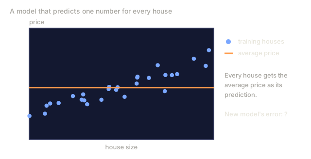
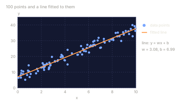
Say you have house sizes and their sale prices, and you want to predict what a new house should sell for given only its size. You could eyeball a trend line on a scatter plot, but eyeballing doesn't scale, and it definitely doesn't turn into code that takes a size and returns a price. What you need is an actual formula: a line that fits the data closely enough to extrapolate from.
That's what linear regression gives you. But the real reason to start here isn't the line. It's that linear regression is your first full pass through the entire ML training loop: define a model, define a cost function, optimize the parameters until the cost stops improving. Most of what's coming later in this phase, logistic regression, SVMs, gradient-boosted ensembles, runs that same three-step pattern with a fancier model and a fancier optimizer bolted on. A few algorithms skip the optimizer step entirely (KNN just measures distances, decision trees split greedily instead of minimizing a cost), but even those still define a model and a criterion for fitting it. Learn the pattern cold on the simplest possible case and you'll recognize it in everything past this phase, too.
Don't mistake simple for small-time. Linear regression runs in production for demand forecasting, A/B test analysis, financial modeling, and as the baseline every fancier regression model has to beat.
The Concept
The Model
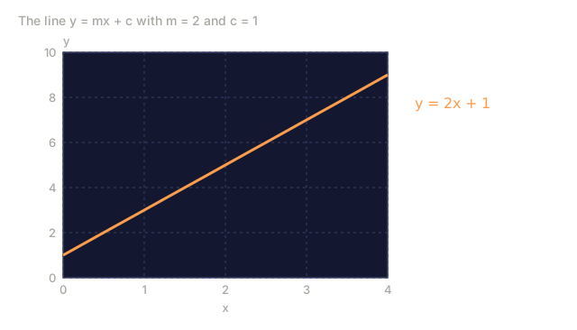
Linear regression assumes a linear relationship between input (x) and output (y):
y = wx + b
w(weight/slope): how much y changes when x increases by 1b(bias/intercept): the value of y when x = 0
With multiple inputs (features), the same idea extends to:
y = w1*x1 + w2*x2 + ... + wn*xn + b
Or in vector form: y = w^T * x + b
The goal: find the w and b that make predicted y land as close as possible to actual y, across every training example at once. Simple to state. Finding it is the rest of this lesson.
The Cost Function (Mean Squared Error)
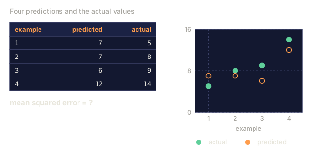
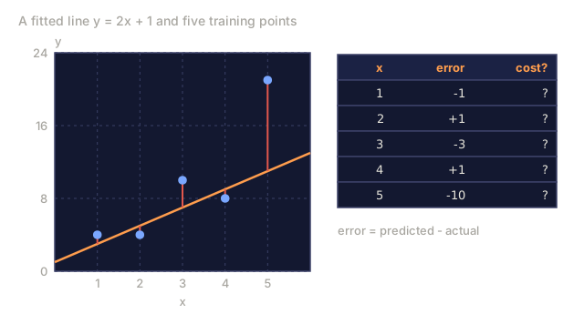
"As close as possible" has to become a single number before you can optimize anything: one score that captures how wrong your predictions are, overall. The standard choice is Mean Squared Error (MSE):
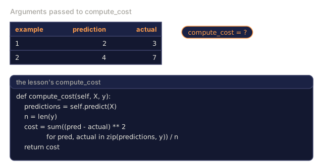
MSE = (1/n) * sum((y_predicted - y_actual)^2)
Why square the error instead of just averaging it? Two reasons. Squaring punishes big misses far harder than small ones: an error of 10 is 100x worse than an error of 1, not 10x. And the squared function is smooth and differentiable everywhere, exactly what an optimizer needs to work with.
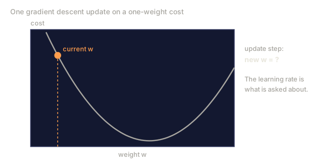
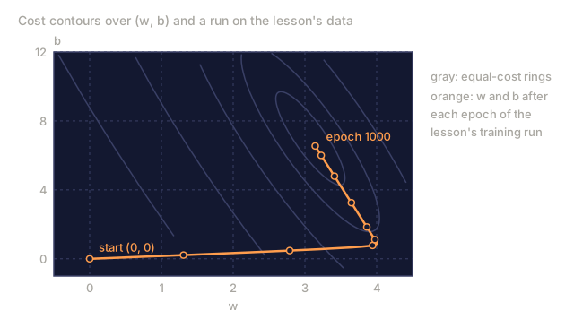
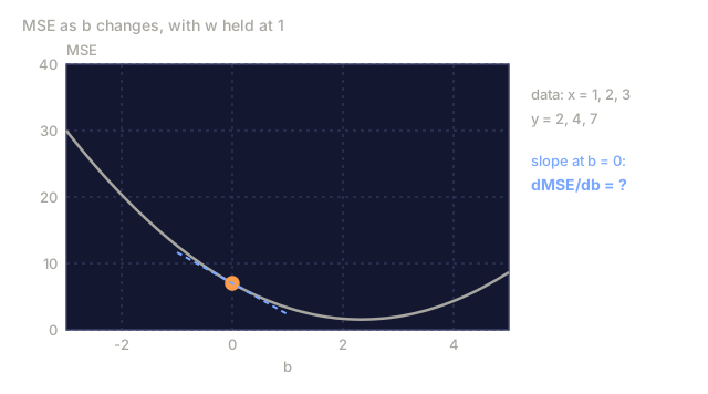
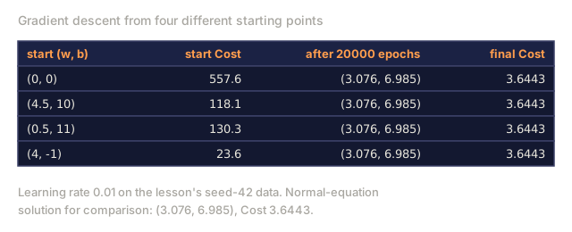
Plot the cost against every possible w and b and you get a surface. For a single weight and bias, that MSE surface is a bowl: a convex paraboloid with one lowest point. Training a linear regression model is nothing more than finding the bottom of that bowl.
Gradient Descent
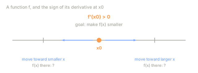
Gradient descent finds the bottom of that bowl by taking steps downhill.

The gradient at each point tells you two things: which direction to move each parameter, and how far.
For MSE with y_hat = wx + b:
dMSE/dw = (2/n) * sum((y_hat - y) * x)
dMSE/db = (2/n) * sum(y_hat - y)
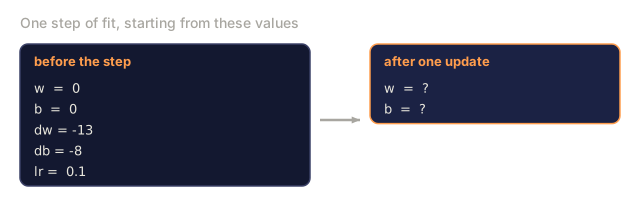
The update rule:
w = w - learning_rate * dMSE/dw
b = b - learning_rate * dMSE/db
The learning rate controls step size, and it's unforgiving in both directions. Too large: you overshoot the minimum and diverge. Too small: training takes forever. Typical starting values: 0.01, 0.001, or 0.0001.
The Normal Equation (Closed-Form Solution)
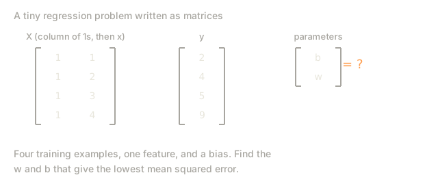
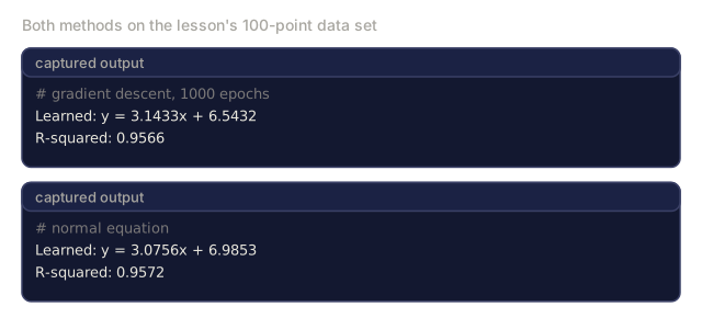
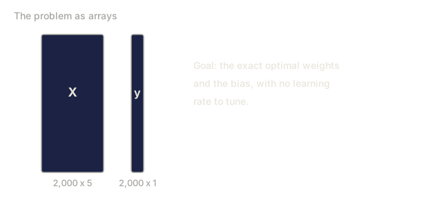
Linear regression has something most ML models don't: a direct formula that hands you the optimal weights with no iteration at all.
w = (X^T * X)^(-1) * X^T * y
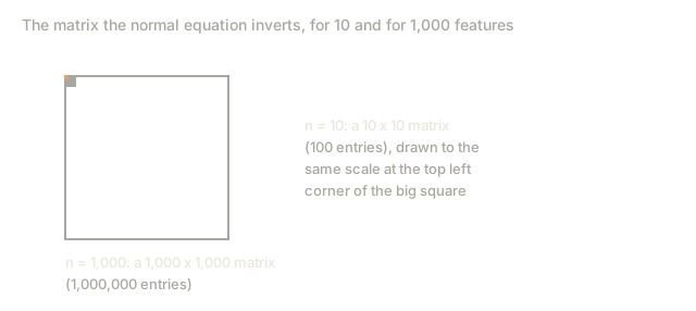
Invert one matrix and you're done. It works great on small datasets. It stops working great on large ones (millions of rows, thousands of features), because matrix inversion costs O(n^3) in the number of features, and gradient descent takes over instead.
Multiple Linear Regression
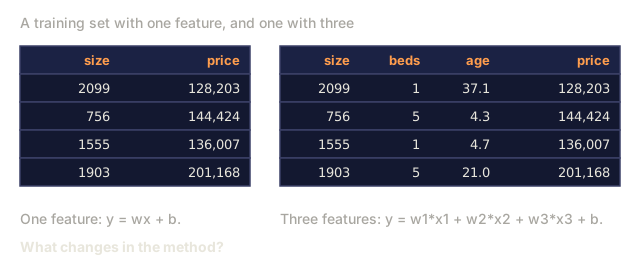
With multiple features, the model becomes:
y = w1*x1 + w2*x2 + ... + wn*xn + b
Nothing about the machinery changes: MSE is still the cost function, gradient descent still updates every weight at once. The only real difference is geometric: you're fitting a hyperplane instead of a line.
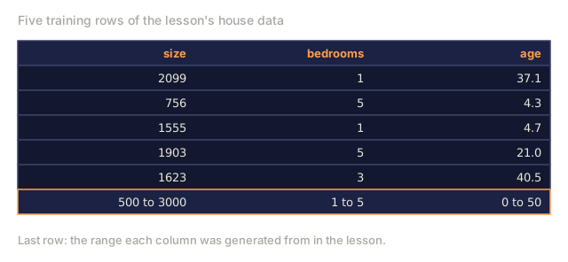
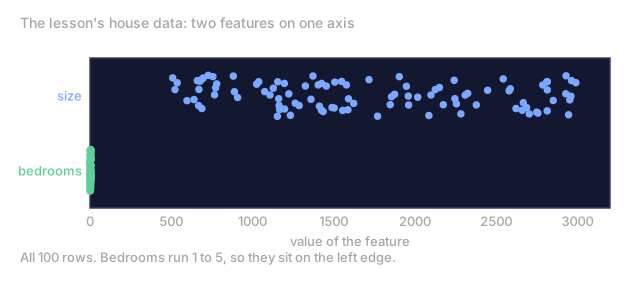
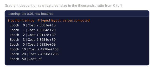
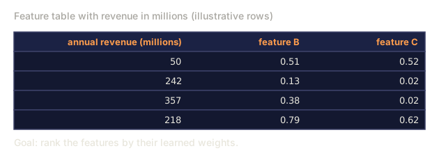
Feature scaling matters more here than it looks like it should. If one feature ranges from 0 to 1 and another ranges from 0 to 1,000,000, the cost surface stretches into a long, thin valley, and gradient descent struggles to navigate it. Standardize your features (subtract the mean, divide by the standard deviation) before training, and the problem disappears.
Polynomial Regression
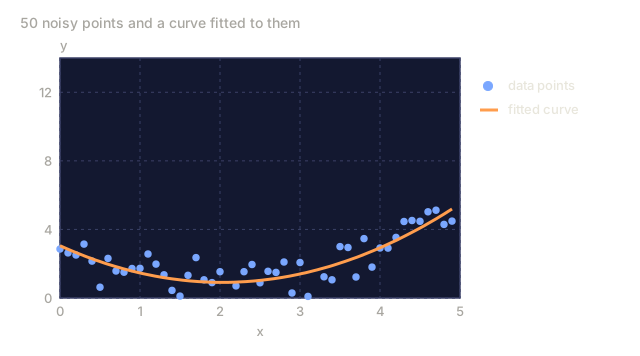
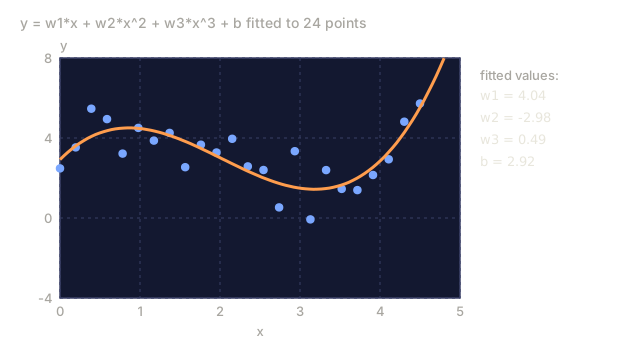
What if the relationship isn't linear? You can still use linear regression, by creating polynomial features instead of raw ones:
y = w1*x + w2*x^2 + w3*x^3 + b
This is still "linear" regression, and the quotes matter: the model is linear in the weights (w1, w2, w3), even though x, x^2, and x^3 aren't. You've just handed it nonlinear features of x and let it fit those instead.
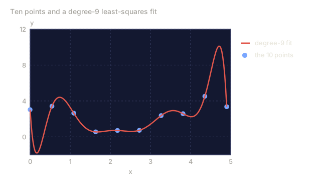
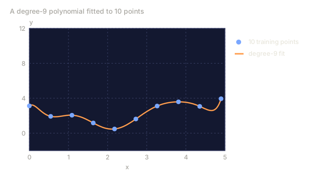
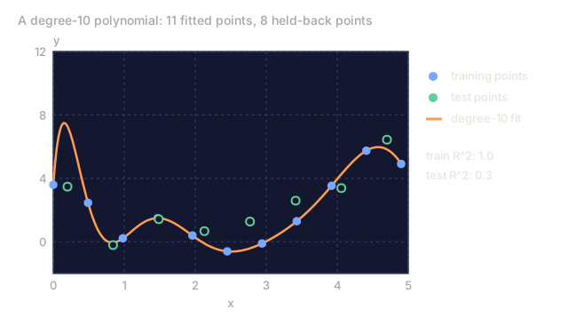
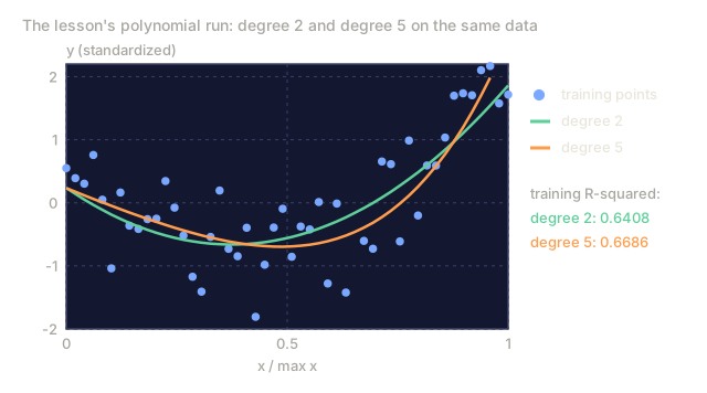
Higher-degree polynomials fit more complex curves, but that power comes at a cost. A degree-10 polynomial will pass through every point in a 10-point dataset and predict poorly on everything that isn't in that dataset.
R-Squared Score
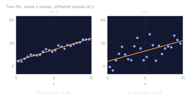
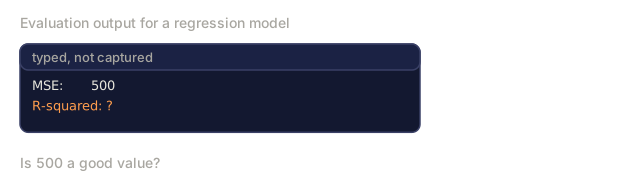
MSE tells you how wrong you are, but the raw number means nothing without knowing the scale of y: is an MSE of 500 good or catastrophic? R-squared (R^2) sidesteps that question entirely with a scale-independent measure:
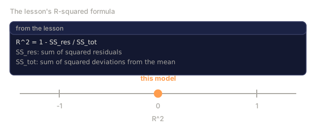
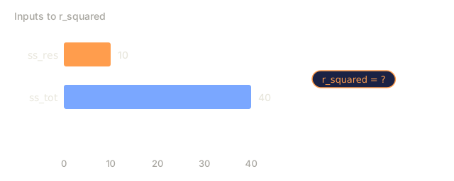
R^2 = 1 - (sum of squared residuals) / (sum of squared deviations from mean)
    = 1 - SS_res / SS_tot
- R^2 = 1.0: perfect predictions
- R^2 = 0.0: no better than predicting the mean every time
- R^2 < 0.0: worse than predicting the mean
Regularization Preview (Ridge Regression)
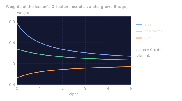
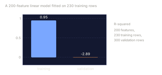
When you have a lot of features, the model can overfit by pushing weights to extreme values. Ridge regression (L2 regularization) heads that off with a penalty added directly to the cost:
Cost = MSE + lambda * sum(w_i^2)
That extra term punishes large weights directly. The hyperparameter lambda sets how hard: higher lambda means smaller weights and more regularization. A later lesson covers this in full; for now, just know it exists and why it helps.
Build It
Step 1: Generate sample data
import random
import math

random.seed(42)

TRUE_W = 3.0
TRUE_B = 7.0
N_SAMPLES = 100

X = [random.uniform(0, 10) for _ in range(N_SAMPLES)]
y = [TRUE_W * x + TRUE_B + random.gauss(0, 2.0) for x in X]

print(f"Generated {N_SAMPLES} samples")
print(f"True relationship: y = {TRUE_W}x + {TRUE_B} (+ noise)")
print(f"First 5 points: {[(round(X[i], 2), round(y[i], 2)) for i in range(5)]}")
Step 2: Linear regression from scratch with gradient descent
class LinearRegression:
    def __init__(self, learning_rate=0.01):
        self.w = 0.0
        self.b = 0.0
        self.lr = learning_rate
        self.cost_history = []

    def predict(self, X):
        return [self.w * x + self.b for x in X]

    def compute_cost(self, X, y):
        predictions = self.predict(X)
        n = len(y)
        cost = sum((pred - actual) ** 2 for pred, actual in zip(predictions, y)) / n
        return cost

    def compute_gradients(self, X, y):
        predictions = self.predict(X)
        n = len(y)
        dw = (2 / n) * sum((pred - actual) * x for pred, actual, x in zip(predictions, y, X))
        db = (2 / n) * sum(pred - actual for pred, actual in zip(predictions, y))
        return dw, db

    def fit(self, X, y, epochs=1000, print_every=200):
        for epoch in range(epochs):
            dw, db = self.compute_gradients(X, y)
            self.w -= self.lr * dw
            self.b -= self.lr * db
            cost = self.compute_cost(X, y)
            self.cost_history.append(cost)
            if epoch % print_every == 0:
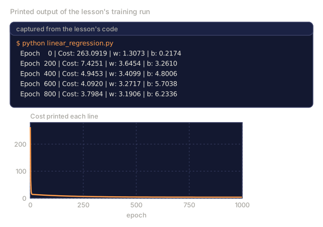
                print(f"  Epoch {epoch:4d} | Cost: {cost:.4f} | w: {self.w:.4f} | b: {self.b:.4f}")
        return self

    def r_squared(self, X, y):
        predictions = self.predict(X)
        y_mean = sum(y) / len(y)
        ss_res = sum((actual - pred) ** 2 for actual, pred in zip(y, predictions))
        ss_tot = sum((actual - y_mean) ** 2 for actual in y)
        return 1 - (ss_res / ss_tot)


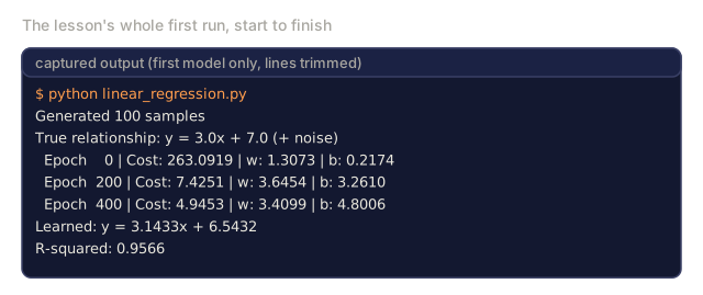
print("=== Training Linear Regression (Gradient Descent) ===")
model = LinearRegression(learning_rate=0.005)
model.fit(X, y, epochs=1000, print_every=200)
print(f"\nLearned: y = {model.w:.4f}x + {model.b:.4f}")
print(f"True:    y = {TRUE_W}x + {TRUE_B}")
print(f"R-squared: {model.r_squared(X, y):.4f}")
Step 3: Normal equation (closed-form solution)
class LinearRegressionNormal:
    def __init__(self):
        self.w = 0.0
        self.b = 0.0

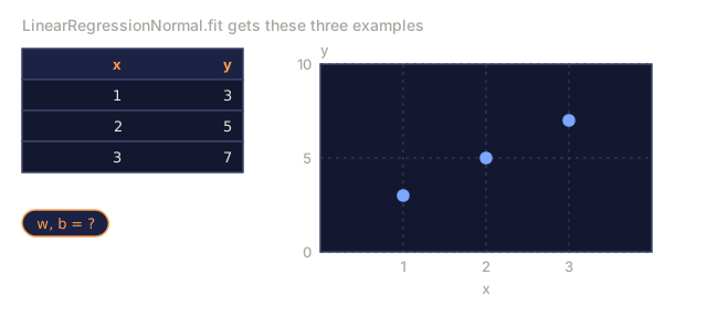
    def fit(self, X, y):
        n = len(X)
        x_mean = sum(X) / n
        y_mean = sum(y) / n
        numerator = sum((X[i] - x_mean) * (y[i] - y_mean) for i in range(n))
        denominator = sum((X[i] - x_mean) ** 2 for i in range(n))
        self.w = numerator / denominator
        self.b = y_mean - self.w * x_mean
        return self

    def predict(self, X):
        return [self.w * x + self.b for x in X]

    def r_squared(self, X, y):
        predictions = self.predict(X)
        y_mean = sum(y) / len(y)
        ss_res = sum((actual - pred) ** 2 for actual, pred in zip(y, predictions))
        ss_tot = sum((actual - y_mean) ** 2 for actual in y)
        return 1 - (ss_res / ss_tot)


print("\n=== Normal Equation (Closed-Form) ===")
model_normal = LinearRegressionNormal()
model_normal.fit(X, y)
print(f"Learned: y = {model_normal.w:.4f}x + {model_normal.b:.4f}")
print(f"R-squared: {model_normal.r_squared(X, y):.4f}")
Step 4: Multiple linear regression
class MultipleLinearRegression:
    def __init__(self, n_features, learning_rate=0.01):
        self.weights = [0.0] * n_features
        self.bias = 0.0
        self.lr = learning_rate
        self.cost_history = []

    def predict_single(self, x):
        return sum(w * xi for w, xi in zip(self.weights, x)) + self.bias

    def predict(self, X):
        return [self.predict_single(x) for x in X]

    def compute_cost(self, X, y):
        predictions = self.predict(X)
        n = len(y)
        return sum((pred - actual) ** 2 for pred, actual in zip(predictions, y)) / n

    def fit(self, X, y, epochs=1000, print_every=200):
        n = len(y)
        n_features = len(X[0])
        for epoch in range(epochs):
            predictions = self.predict(X)
            errors = [pred - actual for pred, actual in zip(predictions, y)]
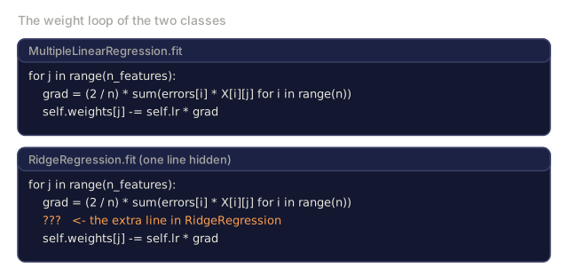
            for j in range(n_features):
                grad = (2 / n) * sum(errors[i] * X[i][j] for i in range(n))
                self.weights[j] -= self.lr * grad
            grad_b = (2 / n) * sum(errors)
            self.bias -= self.lr * grad_b
            cost = self.compute_cost(X, y)
            self.cost_history.append(cost)
            if epoch % print_every == 0:
                print(f"  Epoch {epoch:4d} | Cost: {cost:.4f}")
        return self

    def r_squared(self, X, y):
        predictions = self.predict(X)
        y_mean = sum(y) / len(y)
        ss_res = sum((actual - pred) ** 2 for actual, pred in zip(y, predictions))
        ss_tot = sum((actual - y_mean) ** 2 for actual in y)
        return 1 - (ss_res / ss_tot)


random.seed(42)
N = 100
X_multi = []
y_multi = []
for _ in range(N):
    size = random.uniform(500, 3000)
    bedrooms = random.randint(1, 5)
    age = random.uniform(0, 50)
    price = 50 * size + 10000 * bedrooms - 1000 * age + 50000 + random.gauss(0, 20000)
    X_multi.append([size, bedrooms, age])
    y_multi.append(price)


def standardize(X):
    n_features = len(X[0])
    means = [sum(X[i][j] for i in range(len(X))) / len(X) for j in range(n_features)]
    stds = []
    for j in range(n_features):
        variance = sum((X[i][j] - means[j]) ** 2 for i in range(len(X))) / len(X)
        stds.append(variance ** 0.5)
    X_scaled = []
    for i in range(len(X)):
        row = [(X[i][j] - means[j]) / stds[j] if stds[j] > 0 else 0 for j in range(n_features)]
        X_scaled.append(row)
    return X_scaled, means, stds


y_mean_val = sum(y_multi) / len(y_multi)
y_std_val = (sum((yi - y_mean_val) ** 2 for yi in y_multi) / len(y_multi)) ** 0.5
y_scaled = [(yi - y_mean_val) / y_std_val for yi in y_multi]

X_scaled, x_means, x_stds = standardize(X_multi)

print("\n=== Multiple Linear Regression (3 features) ===")
print("Features: house size, bedrooms, age")
multi_model = MultipleLinearRegression(n_features=3, learning_rate=0.01)
multi_model.fit(X_scaled, y_scaled, epochs=1000, print_every=200)

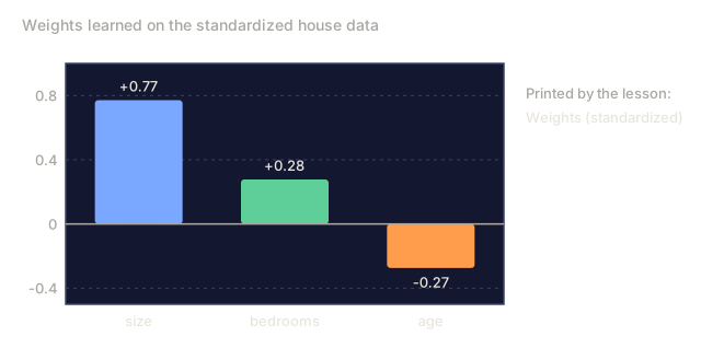
print(f"\nWeights (standardized): {[round(w, 4) for w in multi_model.weights]}")
print(f"Bias (standardized): {multi_model.bias:.4f}")
print(f"R-squared: {multi_model.r_squared(X_scaled, y_scaled):.4f}")
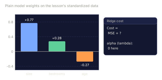
Because every feature was standardized before training, those weights are directly comparable: the largest-magnitude one belongs to whichever feature moves the predicted price the most for a one-standard-deviation change, and its sign gives you the direction. That comparison only works because of the scaling. On raw units, a bigger weight on age than on size wouldn't tell you which feature actually mattered more, a year and a square foot aren't the same unit to begin with.
Step 5: Polynomial regression
class PolynomialRegression:
    def __init__(self, degree, learning_rate=0.01):
        self.degree = degree
        self.weights = [0.0] * degree
        self.bias = 0.0
        self.lr = learning_rate

    def make_features(self, X):
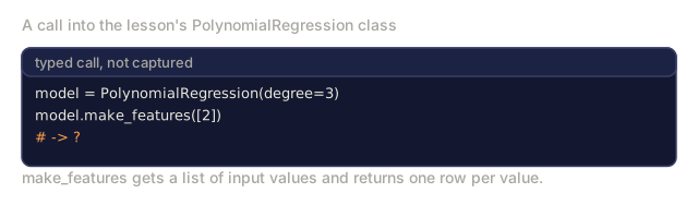
        return [[x ** (d + 1) for d in range(self.degree)] for x in X]

    def predict(self, X):
        features = self.make_features(X)
        return [sum(w * f for w, f in zip(self.weights, row)) + self.bias for row in features]

    def fit(self, X, y, epochs=1000, print_every=200):
        features = self.make_features(X)
        n = len(y)
        for epoch in range(epochs):
            predictions = [sum(w * f for w, f in zip(self.weights, row)) + self.bias for row in features]
            errors = [pred - actual for pred, actual in zip(predictions, y)]
            for j in range(self.degree):
                grad = (2 / n) * sum(errors[i] * features[i][j] for i in range(n))
                self.weights[j] -= self.lr * grad
            grad_b = (2 / n) * sum(errors)
            self.bias -= self.lr * grad_b
            if epoch % print_every == 0:
                cost = sum(e ** 2 for e in errors) / n
                print(f"  Epoch {epoch:4d} | Cost: {cost:.6f}")
        return self

    def r_squared(self, X, y):
        predictions = self.predict(X)
        y_mean = sum(y) / len(y)
        ss_res = sum((actual - pred) ** 2 for actual, pred in zip(y, predictions))
        ss_tot = sum((actual - y_mean) ** 2 for actual in y)
        return 1 - (ss_res / ss_tot)


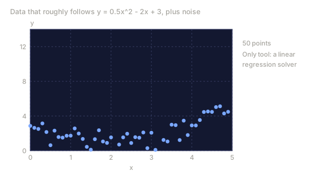
random.seed(42)
X_poly = [x / 10.0 for x in range(0, 50)]
y_poly = [0.5 * x ** 2 - 2 * x + 3 + random.gauss(0, 1.0) for x in X_poly]

x_max = max(abs(x) for x in X_poly)
X_poly_norm = [x / x_max for x in X_poly]
y_poly_mean = sum(y_poly) / len(y_poly)
y_poly_std = (sum((yi - y_poly_mean) ** 2 for yi in y_poly) / len(y_poly)) ** 0.5
y_poly_norm = [(yi - y_poly_mean) / y_poly_std for yi in y_poly]

print("\n=== Polynomial Regression (degree 2 vs degree 5) ===")
print("True relationship: y = 0.5x^2 - 2x + 3")

print("\nDegree 2:")
poly2 = PolynomialRegression(degree=2, learning_rate=0.1)
poly2.fit(X_poly_norm, y_poly_norm, epochs=2000, print_every=500)
print(f"  R-squared: {poly2.r_squared(X_poly_norm, y_poly_norm):.4f}")

print("\nDegree 5:")
poly5 = PolynomialRegression(degree=5, learning_rate=0.1)
poly5.fit(X_poly_norm, y_poly_norm, epochs=2000, print_every=500)
print(f"  R-squared: {poly5.r_squared(X_poly_norm, y_poly_norm):.4f}")

print("\nDegree 2 fits the true curve well. Degree 5 fits training data slightly better")
print("but risks overfitting on new data.")
Step 6: Ridge regression (L2 regularization)
class RidgeRegression:
    def __init__(self, n_features, learning_rate=0.01, alpha=1.0):
        self.weights = [0.0] * n_features
        self.bias = 0.0
        self.lr = learning_rate
        self.alpha = alpha

    def predict_single(self, x):
        return sum(w * xi for w, xi in zip(self.weights, x)) + self.bias

    def predict(self, X):
        return [self.predict_single(x) for x in X]

    def fit(self, X, y, epochs=1000, print_every=200):
        n = len(y)
        n_features = len(X[0])
        for epoch in range(epochs):
            predictions = self.predict(X)
            errors = [pred - actual for pred, actual in zip(predictions, y)]
            mse = sum(e ** 2 for e in errors) / n
            reg_term = self.alpha * sum(w ** 2 for w in self.weights)
            cost = mse + reg_term
            for j in range(n_features):
                grad = (2 / n) * sum(errors[i] * X[i][j] for i in range(n))
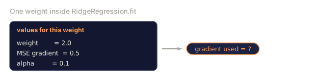
                grad += 2 * self.alpha * self.weights[j]
                self.weights[j] -= self.lr * grad
            grad_b = (2 / n) * sum(errors)
            self.bias -= self.lr * grad_b
            if epoch % print_every == 0:
                print(f"  Epoch {epoch:4d} | Cost: {cost:.4f} | L2 penalty: {reg_term:.4f}")
        return self


print("\n=== Ridge Regression (L2 Regularization) ===")
print("Same data as multiple regression, with alpha=0.1")
ridge = RidgeRegression(n_features=3, learning_rate=0.01, alpha=0.1)
ridge.fit(X_scaled, y_scaled, epochs=1000, print_every=200)
print(f"\nRidge weights: {[round(w, 4) for w in ridge.weights]}")
print(f"Plain weights: {[round(w, 4) for w in multi_model.weights]}")
print("Ridge weights are smaller (shrunk toward zero) due to the L2 penalty.")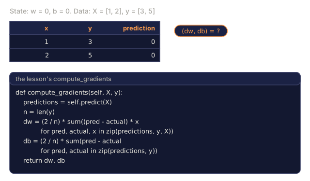
Use It
Now the same thing with scikit-learn, which is what you'll actually reach for in production.
from sklearn.linear_model import LinearRegression as SklearnLR
from sklearn.linear_model import Ridge
from sklearn.preprocessing import PolynomialFeatures, StandardScaler
from sklearn.model_selection import train_test_split
from sklearn.metrics import mean_squared_error, r2_score
import numpy as np

np.random.seed(42)
X_sk = np.random.uniform(0, 10, (100, 1))
y_sk = 3.0 * X_sk.squeeze() + 7.0 + np.random.normal(0, 2.0, 100)

X_train, X_test, y_train, y_test = train_test_split(X_sk, y_sk, test_size=0.2, random_state=42)

lr = SklearnLR()
lr.fit(X_train, y_train)
y_pred = lr.predict(X_test)

print("=== Scikit-learn Linear Regression ===")
print(f"Coefficient (w): {lr.coef_[0]:.4f}")
print(f"Intercept (b): {lr.intercept_:.4f}")
print(f"R-squared (test): {r2_score(y_test, y_pred):.4f}")
print(f"MSE (test): {mean_squared_error(y_test, y_pred):.4f}")

poly = PolynomialFeatures(degree=2, include_bias=False)
X_poly_sk = poly.fit_transform(X_train)
X_poly_test = poly.transform(X_test)

lr_poly = SklearnLR()
lr_poly.fit(X_poly_sk, y_train)
print(f"\nPolynomial degree 2 R-squared: {r2_score(y_test, lr_poly.predict(X_poly_test)):.4f}")

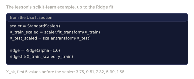
scaler = StandardScaler()
X_train_scaled = scaler.fit_transform(X_train)
X_test_scaled = scaler.transform(X_test)

ridge = Ridge(alpha=1.0)
ridge.fit(X_train_scaled, y_train)
print(f"Ridge R-squared: {r2_score(y_test, ridge.predict(X_test_scaled)):.4f}")
print(f"Ridge coefficient: {ridge.coef_[0]:.4f}")
Your from-scratch version and scikit-learn land on the same numbers. What scikit-learn adds is everything you didn't have to build yourself: edge-case handling, numerical stability, performance tuning. Reach for the library in production. Keep the from-scratch version around for the day you need to know exactly what it's doing under the hood.
Ship It
This lesson produces:
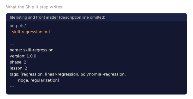
outputs/skill-regression.md, a skill for choosing the right regression approach based on the problem
The instinct once you know scikit-learn exists is to skip straight to LinearRegression().fit() and never touch gradient descent again. Resist that for one more lesson. The point of coding the update rule by hand isn't nostalgia. It's that gradient descent is the optimizer behind almost everything past this point: logistic regression, neural networks, transformers, all of it comes down to some version of "compute a gradient, take a step, repeat." Linear regression is the one place you get to watch that loop with training wheels on, printing w and b every 200 epochs and watching them converge in real time.
The bug I see most often here comes from the learning rate, not the math. Crank it up on unscaled features and MSE doesn't drift upward. It explodes to inf or nan within a few epochs, and the traceback won't tell you why. Nine times out of ten, standardizing your features fixes it faster than shrinking the learning rate ever will. A feature in the thousands sitting next to one between 0 and 1 stretches the cost surface so badly that no single learning rate works well in every direction at once. Scale first, tune the learning rate second, not the other way around.
Exercises
- Implement batch gradient descent, stochastic gradient descent (SGD), and mini-batch gradient descent. Compare convergence speed on the same dataset. Which converges fastest? Which has the smoothest cost curve?
- Generate data from a cubic function (y = ax^3 + bx^2 + cx + d + noise). Fit polynomials of degree 1, 3, and 10. Compare training R^2 and test R^2. At what degree does overfitting become obvious?
- Implement Lasso regression (L1 regularization: penalty = alpha * sum(|w_i|)). Train on the multi-feature housing data. Compare which weights go to zero vs Ridge. Why does L1 produce sparse solutions while L2 doesn't?
Key Terms
| Term | What people say | What it actually means |
|---|---|---|
| Linear regression | "Draw a line through data" | Find weight w and bias b that minimize the sum of squared differences between wx+b and actual y values |
| Cost function | "How bad the model is" | A function that maps model parameters to a single number measuring prediction error, which optimization minimizes |
| Mean squared error | "Average of squared errors" | (1/n) * sum of (predicted - actual)^2, penalizing large errors disproportionately |
| Gradient descent | "Walk downhill" | Iteratively adjust parameters in the direction that reduces the cost function, using partial derivatives |
| Learning rate | "Step size" | A scalar that controls how much parameters change per gradient descent step |
| Normal equation | "Solve it directly" | The closed-form solution w = (X^T X)^-1 X^T y that gives optimal weights without iteration |
| R-squared | "How good the fit is" | The fraction of variance in y explained by the model, ranging from negative infinity to 1.0 |
| Feature scaling | "Make features comparable" | Transforming features to similar ranges (e.g., zero mean, unit variance) so gradient descent converges faster |
| Regularization | "Penalize complexity" | Adding a term to the cost function that shrinks weights, preventing overfitting |
| Ridge regression | "L2 regularization" | Linear regression with a penalty of lambda * sum(w_i^2) added to MSE |
| Polynomial regression | "Fitting curves with linear math" | Linear regression on polynomial features (x, x^2, x^3, ...), still linear in the weights |
| Overfitting | "Memorizing training data" | Using a model so complex that it fits noise in training data and fails on new data |
Further Reading
- An Introduction to Statistical Learning (ISLR) -- free PDF, chapters 3 and 6 cover linear regression and regularization with practical R examples
- The Elements of Statistical Learning (ESL) -- free PDF, the more mathematical companion to ISLR with deeper treatment of ridge and lasso
- Stanford CS229 Lecture Notes on Linear Regression -- Andrew Ng's notes deriving the normal equation and gradient descent from first principles
- scikit-learn LinearRegression documentation -- practical reference for LinearRegression, Ridge, Lasso, and ElasticNet with code examples
Code
- linear_regression.py (python, 344 lines)
- main.jl (text, 292 lines)