Logistic Regression
Logistic regression bends a straight line into an S-curve, so a yes-or-no question gets answered with a probability instead of a guess.
Learning Objectives
- Implement logistic regression from scratch using the sigmoid function and binary cross-entropy loss
- Compute and interpret precision, recall, F1 score, and the confusion matrix for binary classification
- Explain why MSE fails for classification and why binary cross-entropy produces a convex cost surface
- Build a softmax regression model for multi-class classification and evaluate threshold tuning tradeoffs
The Problem
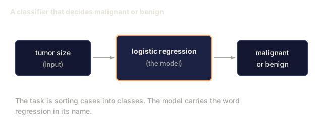
Say you want to predict whether a tumor is malignant or benign from its size. Run linear regression on it and you get numbers like 0.3, or 1.7, or -0.5. None of those mean anything by themselves. Is 1.7 "very malignant"? Is -0.5 "very benign"? Linear regression has no floor and no ceiling, so it will hand you predictions below 0 and above 1 without complaint. Classification needs something narrower: a probability between 0 and 1, plus a clean decision on top of it, yes or no.
That's what logistic regression does. It runs the same linear combination you already know, wx + b, through the sigmoid function, which squeezes any number into the range (0, 1). What comes out the other end is a probability. Pick a threshold, usually 0.5, and you have your decision.
Despite the name, this is a classification algorithm, not a regression one. "Logistic" refers to the sigmoid (logistic) function doing the squeezing; the "regression" part just means you're still fitting weights the same way linear regression does. Confusing name aside, it's one of the most-used algorithms in production ML, precisely because it's this simple.

The Concept
Why Linear Regression Fails for Classification
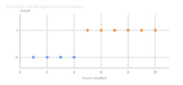
Take a simpler case: predicting pass/fail (1 or 0) from hours studied. Fit a straight line through this data:
hours:  1   2   3   4   5   6   7   8   9   10
actual: 0   0   0   0   1   1   1   1   1   1
and you get predictions like -0.2 at hour 1 and 1.3 at hour 10. Neither is a probability; both sit outside the 0-1 range a yes/no answer needs. Worse, one outlier, say a student who studied for 50 hours, drags the whole line and quietly changes every other prediction along with it.
What classification actually needs is a function that:
- Stays inside 0 and 1, so the output reads as a probability
- Creates a sharp transition: a real decision boundary
- Doesn't get bent out of shape by a stray outlier
The Sigmoid Function
The sigmoid function is exactly that function:
sigmoid(z) = 1 / (1 + e^(-z))
A few properties worth knowing cold:
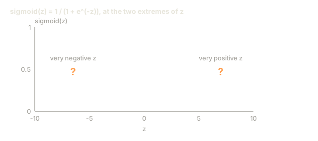
- Large positive z pushes sigmoid(z) toward 1
- Large negative z pushes it toward 0
- z = 0 lands exactly at 0.5
- The output never leaves (0, 1)
- It's smooth and differentiable everywhere: no kinks, no gaps
Its derivative has an unusually clean form: sigmoid'(z) = sigmoid(z) * (1 - sigmoid(z)). That's what makes the gradient computation below cheap.
Logistic Regression = Linear Model + Sigmoid
The model itself is nothing new: compute z = wx + b, exactly like linear regression, then run it through sigmoid.

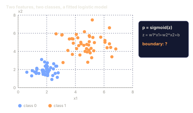
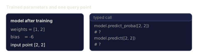
Read the output p as P(y=1 | x): the probability the input belongs to class 1. The decision boundary sits wherever wx + b = 0, because that's the one point where sigmoid outputs exactly 0.5, the fence between the two classes.
Binary Cross-Entropy Loss
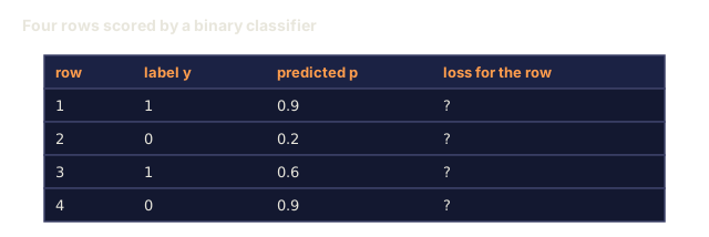
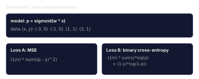
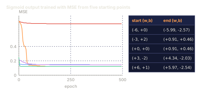
MSE is off the table here. Pair it with sigmoid and the cost surface turns non-convex, riddled with local minima gradient descent can get stuck in. Binary cross-entropy, also called log loss, is the replacement:
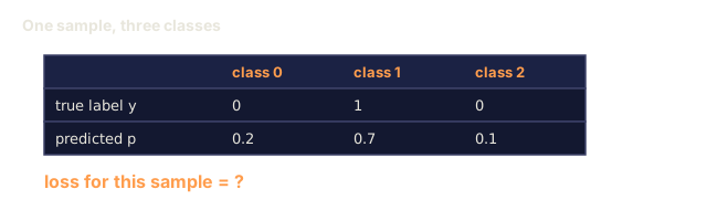
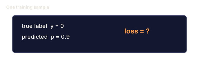
Loss = -(1/n) * sum(y * log(p) + (1-y) * log(1-p))
Walk through why it behaves:
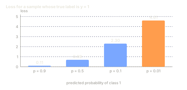
- y=1, p near 1: log(1) = 0, loss near 0. Correct call, low cost.
- y=1, p near 0: log(0) shoots toward negative infinity, loss is enormous. Wrong call, and it pays for it.
- y=0, p near 0: log(1) = 0, loss near 0. Correct call again.
- y=0, p near 1: same blowup, mirrored.
For logistic regression specifically, this loss is convex. One global minimum, no local traps to get stuck in.
Gradient Descent for Logistic Regression
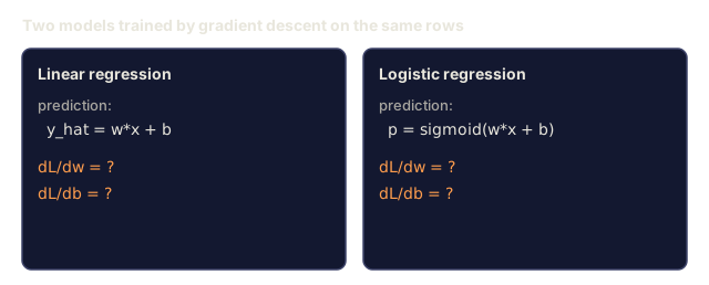
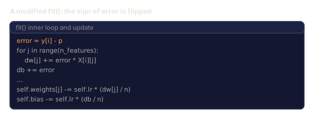
Differentiate binary cross-entropy through sigmoid and the gradients come out clean:
dL/dw = (1/n) * sum((p - y) * x)
dL/db = (1/n) * sum(p - y)
Line these up against the linear regression gradients and you'll notice they're the same shape. The only thing that changed is what p is: sigmoid(wx + b) instead of the raw wx + b. Sigmoid supplies the nonlinearity; the update rule doesn't need to know or care.

The Decision Boundary
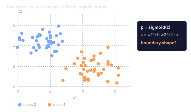
With two features, the decision boundary is just a line:
w1*x1 + w2*x2 + b = 0
Land on one side and the model calls you a 1; land on the other and it calls you a 0. That boundary is always linear, no exceptions, because it's exactly where a linear expression crosses zero. Need a curved boundary instead? Add polynomial features, or use a model that isn't linear to begin with.
Multi-Class Classification with Softmax
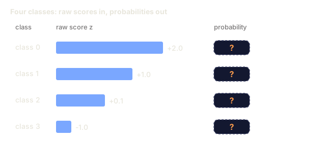
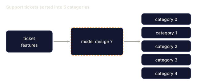
Binary logistic regression tops out at two classes. Once you need k of them, softmax takes over:
softmax(z_i) = e^(z_i) / sum(e^(z_j) for all j)
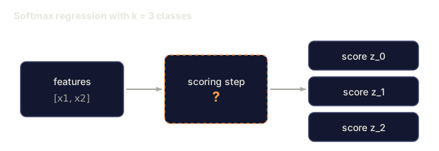
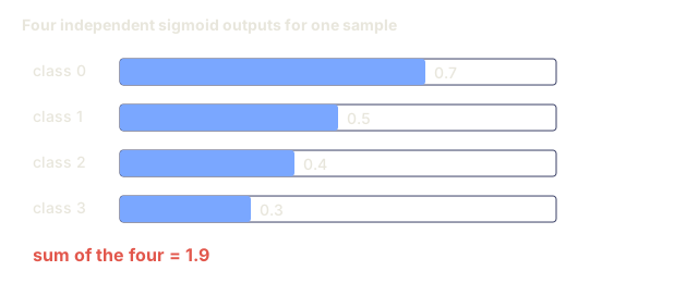
Every class gets its own weight vector and its own raw score z_i. Softmax turns that whole vector of scores into probabilities that sum to 1, and the predicted class is whichever one comes out on top.
The loss becomes categorical cross-entropy:
Loss = -(1/n) * sum(sum(y_k * log(p_k)))
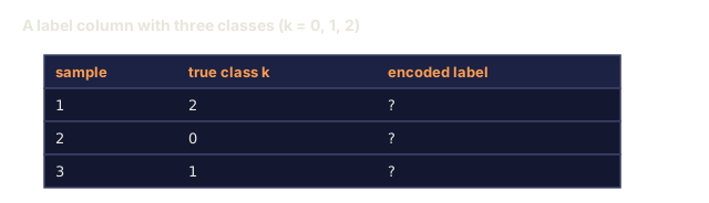
where y_k is 1 for the true class and 0 everywhere else: the one-hot encoding of the label.
Evaluation Metrics
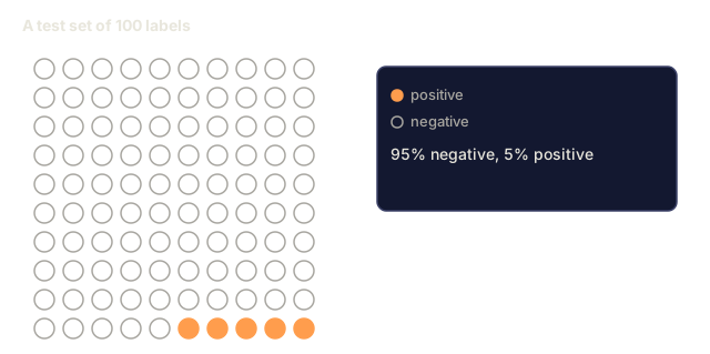
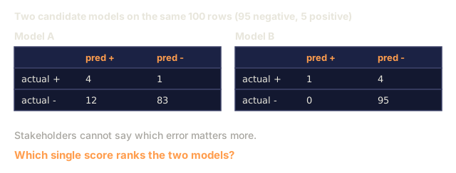
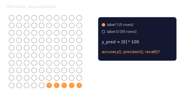
Accuracy by itself will lie to you. Take a dataset that's 95% negative and 5% positive: a model that predicts negative every single time still scores 95% accuracy, and does zero useful work.
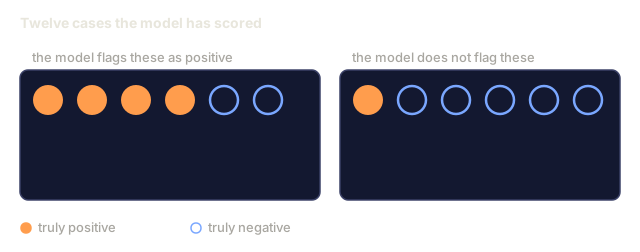
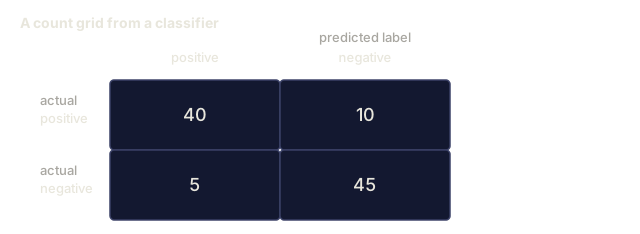
Confusion Matrix:
| Predicted Positive | Predicted Negative | |
|---|---|---|
| Actually Positive | True Positive (TP) | False Negative (FN) |
| Actually Negative | False Positive (FP) | True Negative (TN) |
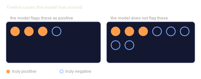
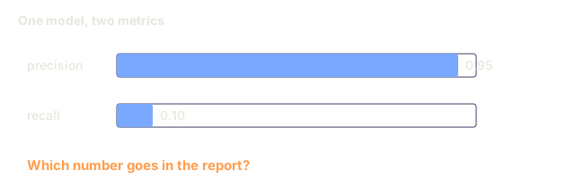
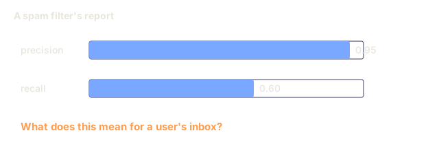
Precision: of everything the model flagged as positive, how much actually was?
Precision = TP / (TP + FP)
Recall (Sensitivity): of everything that actually was positive, how much did the model catch?
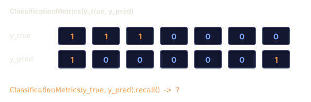
Recall = TP / (TP + FN)
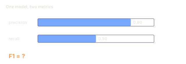
F1 Score: the harmonic mean of the two, one number that won't let either metric hide.
F1 = 2 * (Precision * Recall) / (Precision + Recall)
Which one to chase depends on what a mistake costs:
- Precision, when false positives are expensive: a spam filter that nukes real email is worse than one that lets a little spam through.
- Recall, when false negatives are expensive: a cancer screen that misses a tumor is worse than one that raises a false alarm.
- F1, when you need a single number and can't afford to pick a side.



Build It
Step 1: Sigmoid function and data generation
import random
import math

def sigmoid(z):
    z = max(-500, min(500, z))
    return 1.0 / (1.0 + math.exp(-z))


random.seed(42)
N = 200
X = []
y = []

for _ in range(N // 2):
    X.append([random.gauss(2, 1), random.gauss(2, 1)])
    y.append(0)

for _ in range(N // 2):
    X.append([random.gauss(5, 1), random.gauss(5, 1)])
    y.append(1)

combined = list(zip(X, y))
random.shuffle(combined)
X, y = zip(*combined)
X = list(X)
y = list(y)

print(f"Generated {N} samples (2 classes, 2 features)")
print(f"Class 0 center: (2, 2), Class 1 center: (5, 5)")
print(f"First 5 samples:")
for i in range(5):
    print(f"  Features: [{X[i][0]:.2f}, {X[i][1]:.2f}], Label: {y[i]}")
Step 2: Logistic regression from scratch
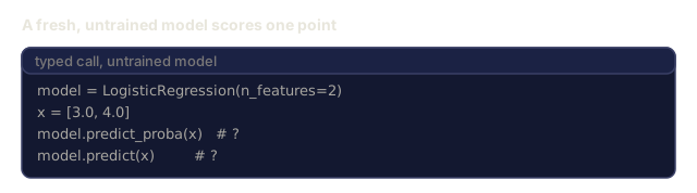
class LogisticRegression:
    def __init__(self, n_features, learning_rate=0.01):
        self.weights = [0.0] * n_features
        self.bias = 0.0
        self.lr = learning_rate
        self.loss_history = []

    def predict_proba(self, x):
        z = sum(w * xi for w, xi in zip(self.weights, x)) + self.bias
        return sigmoid(z)

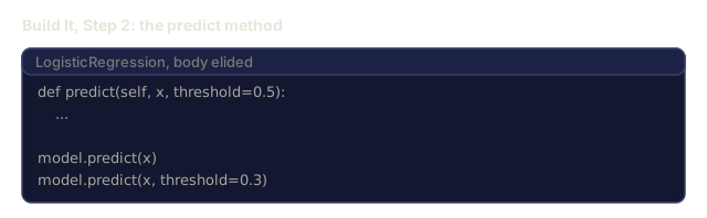
    def predict(self, x, threshold=0.5):
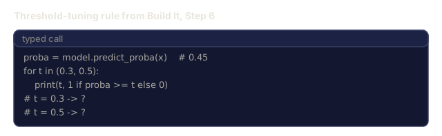
        return 1 if self.predict_proba(x) >= threshold else 0

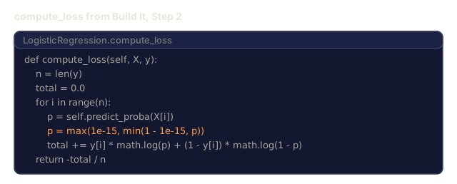
    def compute_loss(self, X, y):
        n = len(y)
        total = 0.0
        for i in range(n):
            p = self.predict_proba(X[i])
            p = max(1e-15, min(1 - 1e-15, p))
            total += y[i] * math.log(p) + (1 - y[i]) * math.log(1 - p)
        return -total / n

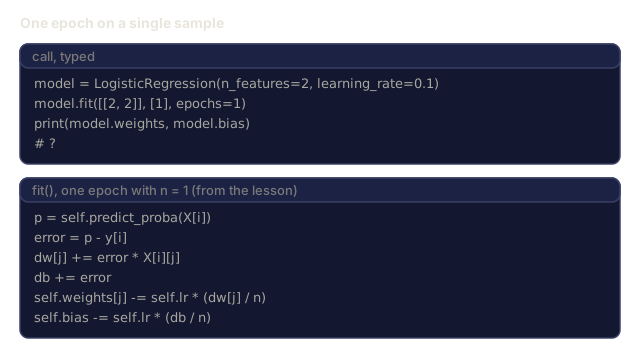
    def fit(self, X, y, epochs=1000, print_every=200):
        n = len(y)
        n_features = len(X[0])
        for epoch in range(epochs):
            dw = [0.0] * n_features
            db = 0.0
            for i in range(n):
                p = self.predict_proba(X[i])
                error = p - y[i]
                for j in range(n_features):
                    dw[j] += error * X[i][j]
                db += error
            for j in range(n_features):
                self.weights[j] -= self.lr * (dw[j] / n)
            self.bias -= self.lr * (db / n)
            loss = self.compute_loss(X, y)
            self.loss_history.append(loss)
            if epoch % print_every == 0:
                print(f"  Epoch {epoch:4d} | Loss: {loss:.4f} | w: [{self.weights[0]:.3f}, {self.weights[1]:.3f}] | b: {self.bias:.3f}")
        return self

    def accuracy(self, X, y):
        correct = sum(1 for i in range(len(y)) if self.predict(X[i]) == y[i])
        return correct / len(y)


split = int(0.8 * N)
X_train, X_test = X[:split], X[split:]
y_train, y_test = y[:split], y[split:]

print("\n=== Training Logistic Regression ===")
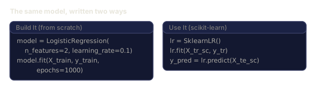
model = LogisticRegression(n_features=2, learning_rate=0.1)
model.fit(X_train, y_train, epochs=1000, print_every=200)

print(f"\nTrain accuracy: {model.accuracy(X_train, y_train):.4f}")
print(f"Test accuracy:  {model.accuracy(X_test, y_test):.4f}")
print(f"Weights: [{model.weights[0]:.4f}, {model.weights[1]:.4f}]")
print(f"Bias: {model.bias:.4f}")
Step 3: Confusion matrix and metrics from scratch
class ClassificationMetrics:
    def __init__(self, y_true, y_pred):
        self.tp = sum(1 for t, p in zip(y_true, y_pred) if t == 1 and p == 1)
        self.tn = sum(1 for t, p in zip(y_true, y_pred) if t == 0 and p == 0)
        self.fp = sum(1 for t, p in zip(y_true, y_pred) if t == 0 and p == 1)
        self.fn = sum(1 for t, p in zip(y_true, y_pred) if t == 1 and p == 0)

    def accuracy(self):
        total = self.tp + self.tn + self.fp + self.fn
        return (self.tp + self.tn) / total if total > 0 else 0

    def precision(self):
        denom = self.tp + self.fp
        return self.tp / denom if denom > 0 else 0

    def recall(self):
        denom = self.tp + self.fn
        return self.tp / denom if denom > 0 else 0

    def f1(self):
        p = self.precision()
        r = self.recall()
        return 2 * p * r / (p + r) if (p + r) > 0 else 0

    def print_confusion_matrix(self):
        print(f"\n  Confusion Matrix:")
        print(f"                  Predicted")
        print(f"                  Pos   Neg")
        print(f"  Actual Pos     {self.tp:4d}  {self.fn:4d}")
        print(f"  Actual Neg     {self.fp:4d}  {self.tn:4d}")

    def print_report(self):
        self.print_confusion_matrix()
        print(f"\n  Accuracy:  {self.accuracy():.4f}")
        print(f"  Precision: {self.precision():.4f}")
        print(f"  Recall:    {self.recall():.4f}")
        print(f"  F1 Score:  {self.f1():.4f}")


y_pred_test = [model.predict(x) for x in X_test]
print("\n=== Classification Report (Test Set) ===")
metrics = ClassificationMetrics(y_test, y_pred_test)
metrics.print_report()
Step 4: Decision boundary analysis
print("\n=== Decision Boundary ===")
w1, w2 = model.weights
b = model.bias
print(f"Decision boundary: {w1:.4f}*x1 + {w2:.4f}*x2 + {b:.4f} = 0")
if abs(w2) > 1e-10:
    print(f"Solved for x2:     x2 = {-w1/w2:.4f}*x1 + {-b/w2:.4f}")

print("\nSample predictions near the boundary:")
test_points = [
    [3.0, 3.0],
    [3.5, 3.5],
    [4.0, 4.0],
    [2.5, 2.5],
    [5.0, 5.0],
]
for point in test_points:
    prob = model.predict_proba(point)
    pred = model.predict(point)
    print(f"  [{point[0]}, {point[1]}] -> prob={prob:.4f}, class={pred}")
Step 5: Multi-class with softmax
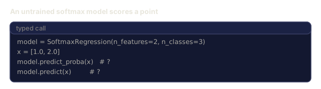
class SoftmaxRegression:
    def __init__(self, n_features, n_classes, learning_rate=0.01):
        self.n_features = n_features
        self.n_classes = n_classes
        self.lr = learning_rate
        self.weights = [[0.0] * n_features for _ in range(n_classes)]
        self.biases = [0.0] * n_classes

    def softmax(self, scores):
        max_score = max(scores)
        exp_scores = [math.exp(s - max_score) for s in scores]
        total = sum(exp_scores)
        return [e / total for e in exp_scores]

    def predict_proba(self, x):
        scores = [
            sum(self.weights[k][j] * x[j] for j in range(self.n_features)) + self.biases[k]
            for k in range(self.n_classes)
        ]
        return self.softmax(scores)

    def predict(self, x):
        probs = self.predict_proba(x)
        return probs.index(max(probs))

    def fit(self, X, y, epochs=1000, print_every=200):
        n = len(y)
        for epoch in range(epochs):
            grad_w = [[0.0] * self.n_features for _ in range(self.n_classes)]
            grad_b = [0.0] * self.n_classes
            total_loss = 0.0
            for i in range(n):
                probs = self.predict_proba(X[i])
                for k in range(self.n_classes):
                    target = 1.0 if y[i] == k else 0.0
                    error = probs[k] - target
                    for j in range(self.n_features):
                        grad_w[k][j] += error * X[i][j]
                    grad_b[k] += error
                true_prob = max(probs[y[i]], 1e-15)
                total_loss -= math.log(true_prob)
            for k in range(self.n_classes):
                for j in range(self.n_features):
                    self.weights[k][j] -= self.lr * (grad_w[k][j] / n)
                self.biases[k] -= self.lr * (grad_b[k] / n)
            if epoch % print_every == 0:
                print(f"  Epoch {epoch:4d} | Loss: {total_loss / n:.4f}")
        return self

    def accuracy(self, X, y):
        correct = sum(1 for i in range(len(y)) if self.predict(X[i]) == y[i])
        return correct / len(y)


random.seed(42)
X_3class = []
y_3class = []

centers = [(1, 1), (5, 1), (3, 5)]
for label, (cx, cy) in enumerate(centers):
    for _ in range(50):
        X_3class.append([random.gauss(cx, 0.8), random.gauss(cy, 0.8)])
        y_3class.append(label)

combined = list(zip(X_3class, y_3class))
random.shuffle(combined)
X_3class, y_3class = zip(*combined)
X_3class = list(X_3class)
y_3class = list(y_3class)

split_3 = int(0.8 * len(X_3class))
X_train_3 = X_3class[:split_3]
y_train_3 = y_3class[:split_3]
X_test_3 = X_3class[split_3:]
y_test_3 = y_3class[split_3:]

print("\n=== Multi-class Softmax Regression (3 classes) ===")
softmax_model = SoftmaxRegression(n_features=2, n_classes=3, learning_rate=0.1)
softmax_model.fit(X_train_3, y_train_3, epochs=1000, print_every=200)
print(f"\nTrain accuracy: {softmax_model.accuracy(X_train_3, y_train_3):.4f}")
print(f"Test accuracy:  {softmax_model.accuracy(X_test_3, y_test_3):.4f}")

print("\nSample predictions:")
for i in range(5):
    probs = softmax_model.predict_proba(X_test_3[i])
    pred = softmax_model.predict(X_test_3[i])
    print(f"  True: {y_test_3[i]}, Predicted: {pred}, Probs: [{', '.join(f'{p:.3f}' for p in probs)}]")
Step 6: Threshold tuning
print("\n=== Threshold Tuning ===")
print("Default threshold: 0.5. Adjusting the threshold trades precision for recall.\n")

thresholds = [0.3, 0.4, 0.5, 0.6, 0.7]
print(f"{'Threshold':>10} {'Accuracy':>10} {'Precision':>10} {'Recall':>10} {'F1':>10}")
print("-" * 52)

for t in thresholds:
    y_pred_t = [1 if model.predict_proba(x) >= t else 0 for x in X_test]
    m = ClassificationMetrics(y_test, y_pred_t)
    print(f"{t:>10.1f} {m.accuracy():>10.4f} {m.precision():>10.4f} {m.recall():>10.4f} {m.f1():>10.4f}")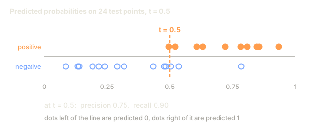

Use It
Now the same model, built with scikit-learn instead of from scratch.
from sklearn.linear_model import LogisticRegression as SklearnLR
from sklearn.metrics import accuracy_score, precision_score, recall_score, f1_score
from sklearn.metrics import confusion_matrix, classification_report
from sklearn.model_selection import train_test_split
from sklearn.preprocessing import StandardScaler
import numpy as np

np.random.seed(42)
X_0 = np.random.randn(100, 2) + [2, 2]
X_1 = np.random.randn(100, 2) + [5, 5]
X_sk = np.vstack([X_0, X_1])
y_sk = np.array([0] * 100 + [1] * 100)

X_tr, X_te, y_tr, y_te = train_test_split(X_sk, y_sk, test_size=0.2, random_state=42)

scaler = StandardScaler()
X_tr_sc = scaler.fit_transform(X_tr)
X_te_sc = scaler.transform(X_te)

lr = SklearnLR()
lr.fit(X_tr_sc, y_tr)
y_pred = lr.predict(X_te_sc)

print("=== Scikit-learn Logistic Regression ===")
print(f"Accuracy:  {accuracy_score(y_te, y_pred):.4f}")
print(f"Precision: {precision_score(y_te, y_pred):.4f}")
print(f"Recall:    {recall_score(y_te, y_pred):.4f}")
print(f"F1:        {f1_score(y_te, y_pred):.4f}")
print(f"\nConfusion Matrix:\n{confusion_matrix(y_te, y_pred)}")
print(f"\nClassification Report:\n{classification_report(y_te, y_pred)}")
Same decision boundary, same metrics, just less code. What scikit-learn buys you on top: solver options (liblinear, lbfgs, saga), regularization built in, multi-class strategies (one-vs-rest, multinomial), and numerical stability you'd otherwise have to earn the hard way.
Ship It
This lesson produces:
code/logistic_regression.py- logistic regression from scratch with metrics
The mistake I see most often isn't in the math, it's in skipping this model entirely. Teams reach for a gradient-boosted tree or a neural net because logistic regression sounds like the beginner option, then burn a week debugging why the fancy model barely clears a coin flip.
Run logistic regression first on every classification problem, even the ones you're sure need something heavier. It trains in seconds, it tells you immediately whether your features carry any signal at all, and it hands you a precision/recall baseline the complicated model actually has to beat, not just match. If the fancy model can't clear that bar, the problem usually isn't the model. It's the features, the labels, or the framing of the task.
Exercises
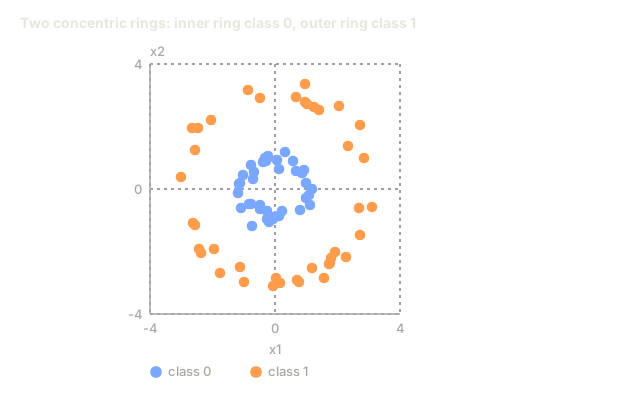
- Generate a dataset that is NOT linearly separable (e.g., two concentric circles). Train logistic regression and observe its failure. Then add polynomial features (x1^2, x2^2, x1*x2) and train again. Show that the accuracy improves.
- Implement a multi-class confusion matrix for the 3-class softmax model. Compute per-class precision and recall. Which class is hardest to classify?
- Build an ROC curve from scratch. For 100 threshold values from 0 to 1, compute the true positive rate and false positive rate. Calculate the AUC (area under the curve) using the trapezoidal rule.
Key Terms
| Term | What people say | What it actually means |
|---|---|---|
| Logistic regression | "Regression for classification" | A linear model followed by a sigmoid function that outputs class probabilities |
| Sigmoid function | "The S-curve" | The function 1/(1+e^(-z)) that maps any real number to the range (0, 1) |
| Binary cross-entropy | "Log loss" | The loss function -[y*log(p) + (1-y)*log(1-p)] that penalizes confident wrong predictions severely |
| Decision boundary | "The dividing line" | The surface where the model's output probability equals 0.5, separating predicted classes |
| Softmax | "Multi-class sigmoid" | A function that converts a vector of scores into probabilities that sum to 1 |
| Precision | "How many selected are relevant" | TP / (TP + FP), the fraction of positive predictions that are actually positive |
| Recall | "How many relevant are selected" | TP / (TP + FN), the fraction of actual positives that the model correctly identifies |
| F1 score | "Balanced accuracy" | The harmonic mean of precision and recall: 2PR / (P+R) |
| Confusion matrix | "The error breakdown" | A table showing TP, TN, FP, FN counts for each class pair |
| Threshold | "The cutoff" | The probability value above which the model predicts class 1 (default 0.5, tunable) |
| One-hot encoding | "Binary columns for categories" | Representing class k as a vector of zeros with a 1 at position k |
| Categorical cross-entropy | "Multi-class log loss" | The extension of binary cross-entropy to k classes using one-hot encoded labels |
Code
- logistic_regression.py (python, 326 lines)
- main.jl (text, 386 lines)