Image Classification
A classifier is a function from pixels to a probability distribution over classes. Everything else is plumbing.
Learning Objectives
- Build an end-to-end image classification pipeline on CIFAR-10: dataset, augmentation, model, training loop, evaluation
- Explain the role of each component (dataloader, loss, optimizer, scheduler, augmentation) and predict how breaking any one of them manifests in the loss curve
- Implement mixup from scratch, apply label smoothing, and explain how cutmix and Cutout work well enough to justify when each is worth adding
- Read a confusion matrix and a per-class precision/recall table to diagnose dataset and model failures beyond aggregate accuracy
The Problem
Every vision task that ships reduces to image classification at some level. Detection classifies regions. Segmentation classifies pixels. Retrieval ranks by similarity to class centroids. Getting classification right (the dataset loop, the augmentation policy, the loss, the evaluation) is the skill that transfers to every other task in this phase.
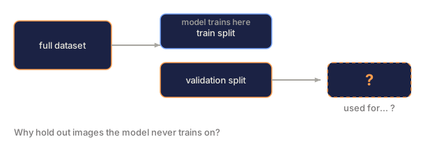
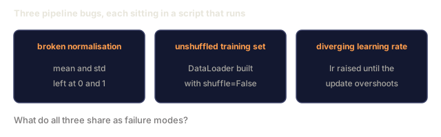
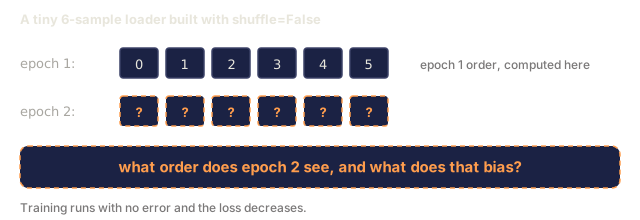
Most classification bugs are not in the model. They live in the pipeline: a broken normalisation, an unshuffled training set, augmentation that distorts labels, a validation split contaminated by training data, a learning rate that silently diverges after epoch 30. A CNN that would hit 93% on CIFAR-10 with a correct setup commonly scores 70-75% with a broken one, and the loss curve looks plausible the whole time.
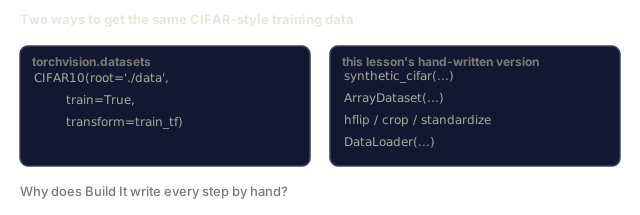
This lesson wires the entire pipeline by hand so every part is inspectable. You will not touch torchvision.datasets in Build It, because that is exactly where a bug likes to hide when you can't see inside it.
The Concept
The classification pipeline

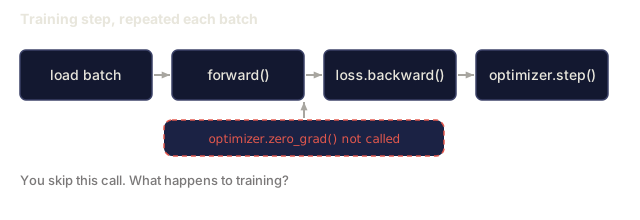
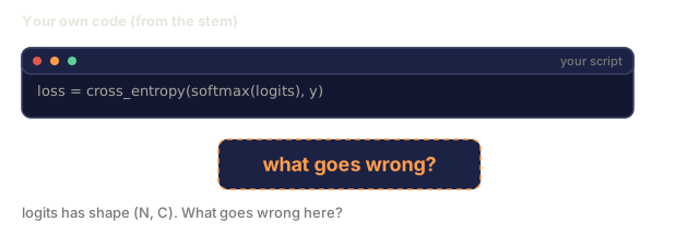
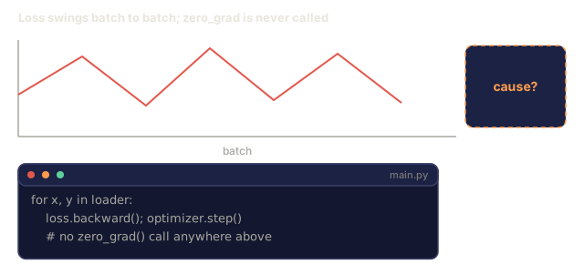
Every line in this loop is where a bug can live. Cross-entropy takes raw logits, not softmax outputs, so any model(x).softmax() before the loss quietly computes the wrong gradient. Augmentations apply to inputs only, not labels, except for mixup, which mixes both. optimizer.zero_grad() must happen once per step: skip it and gradients accumulate, which looks exactly like a wildly unstable learning rate. Each of those bugs flattens the learning curve without ever throwing an error.
Cross-entropy, logits, and softmax
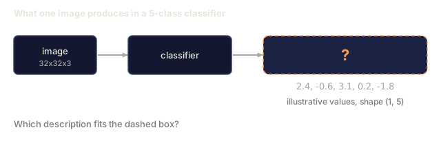
A classifier produces C numbers per image called logits. Applying softmax converts them into a probability distribution:
softmax(z)_i = exp(z_i) / sum_j exp(z_j)
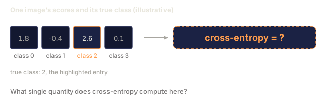
Cross-entropy measures the negative log probability of the correct class:
CE(z, y) = -log( softmax(z)_y )
        = -z_y + log( sum_j exp(z_j) )
The right-hand form is the numerically stable one (log-sum-exp). PyTorch's nn.CrossEntropyLoss fuses softmax + NLL in one op and takes raw logits directly. Applying softmax yourself first is almost always a bug: you end up computing log(softmax(softmax(z))), a meaningless quantity.
Why augmentation works
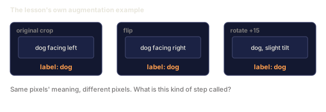
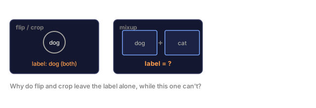
Augmentation is any pixel-level transform applied to a training image (a crop, a flip, a colour shift) that leaves the image's label unchanged. A CNN has inductive bias for translation (from weight sharing) but no built-in invariance to crops, flips, colour jitter, or occlusion. The only way to teach it those invariances is to show it pixels that exercise them. Every random transform during training is a way of saying: "these two images have the same label; learn the features that ignore the difference."
Original crop:  "dog facing left"
Flip:           "dog facing right"       <- same label, different pixels
Rotate(+15):    "dog, slight tilt"
Colour jitter:  "dog in warmer light"
RandomErasing:  "dog with patch missing"
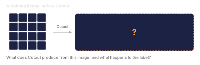
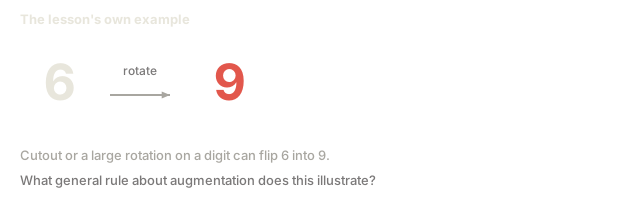
The rule: augmentation must preserve the label. Cutout (zeroing out a random square patch of the image) and rotation on a digit can flip "6" into "9"; for that dataset you use smaller rotation ranges and pick augmentations that respect digit-specific invariances.
Mixup and cutmix
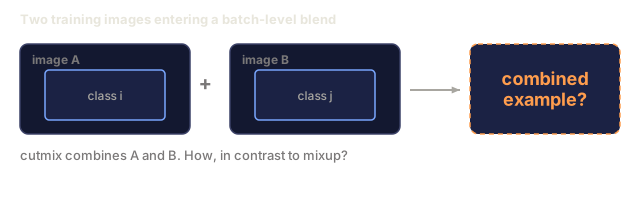
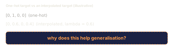
Ordinary augmentation transforms pixels but keeps labels one-hot. Mixup and cutmix break that by interpolating both.
Mixup:
  lambda ~ Beta(a, a)
  x = lambda * x_i + (1 - lambda) * x_j
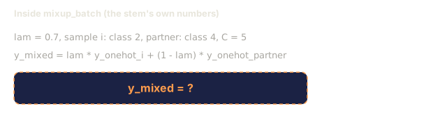
  y = lambda * y_i + (1 - lambda) * y_j

Cutmix:
  paste a random rectangle of x_j into x_i
  y = area-weighted mix of y_i and y_j
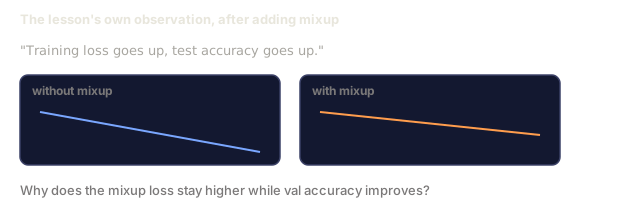
Why it helps: the model stops memorising spiky one-hot targets and learns to interpolate between classes. Training loss goes up, test accuracy goes up. It is the single cheapest robustness upgrade for any classifier.
Label smoothing
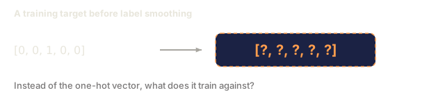
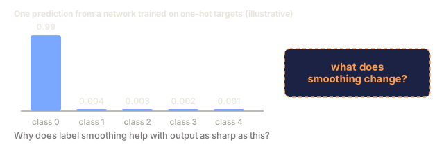
A cousin of mixup. Instead of training against [0, 0, 1, 0, 0], train against [eps/C, eps/C, 1-eps, eps/C, eps/C] for a small eps like 0.1. Stops the model from producing arbitrarily sharp logits and improves calibration at almost no cost. Built into nn.CrossEntropyLoss(label_smoothing=0.1) since PyTorch 1.10.
Evaluation beyond accuracy
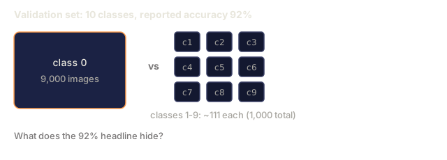
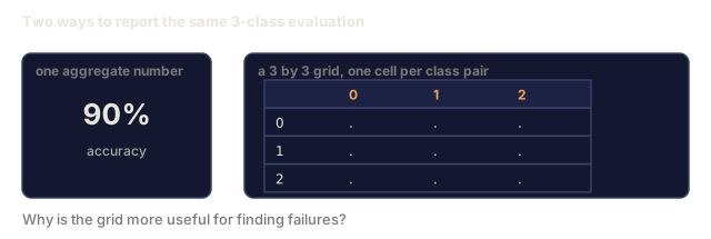
Aggregate accuracy hides imbalance. A 90-10 binary classifier that always predicts the majority class scores 90%. The tools that actually tell you what is happening:
- Per-class accuracy: one number per class, so it immediately surfaces underperforming categories.
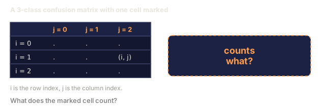
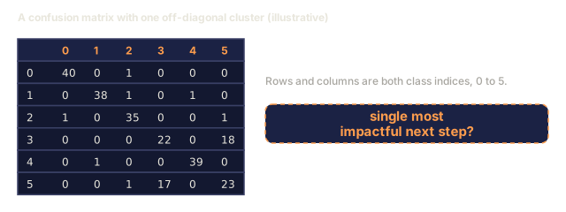
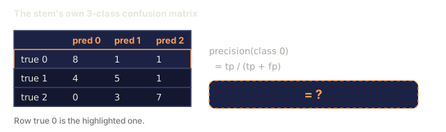
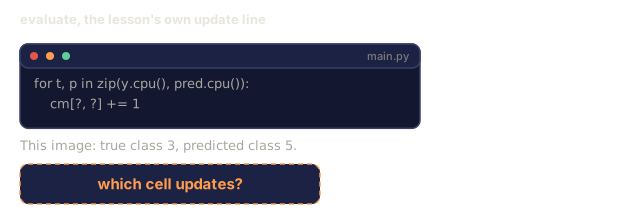
- Confusion matrix: a C x C grid where row i, column j counts how many true-class-i images got predicted as class j. The diagonal is correct; the off-diagonals are where your model actually lives.
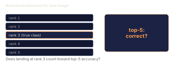
- Top-1 / Top-5: whether the correct class lands in the top 1 or top 5 predictions. Top-5 matters for ImageNet because classes like "Norwich terrier" vs "Norfolk terrier" are genuinely ambiguous.
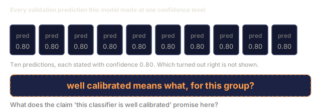
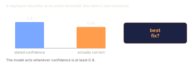
- Calibration (ECE, expected calibration error): does a prediction with 0.8 confidence turn out right 80% of the time? Modern networks are systematically over-confident, so fix it with temperature scaling or label smoothing.




Build It
Step 1: A deterministic synthetic dataset
CIFAR-10 lives on disk. To make this lesson reproducible and fast we build a synthetic dataset that looks like CIFAR: 32x32 RGB images with class-specific structure the model must learn. The exact same pipeline works unchanged on real CIFAR-10.
import numpy as np
import torch
from torch.utils.data import Dataset


def synthetic_cifar(num_per_class=1000, num_classes=10, seed=0):
    rng = np.random.default_rng(seed)
    X = []
    Y = []
    for c in range(num_classes):
        centre = rng.uniform(0, 1, (3,))
        freq = 2 + c
        for _ in range(num_per_class):
            yy, xx = np.meshgrid(np.linspace(0, 1, 32), np.linspace(0, 1, 32), indexing="ij")
            r = np.sin(xx * freq) * 0.5 + centre[0]
            g = np.cos(yy * freq) * 0.5 + centre[1]
            b = (xx + yy) * 0.5 * centre[2]
            img = np.stack([r, g, b], axis=-1)
            img += rng.normal(0, 0.08, img.shape)
            img = np.clip(img, 0, 1)
            X.append(img.astype(np.float32))
            Y.append(c)
    X = np.stack(X)
    Y = np.array(Y)
    idx = rng.permutation(len(X))
    return X[idx], Y[idx]


class ArrayDataset(Dataset):
    def __init__(self, X, Y, transform=None):
        self.X = X
        self.Y = Y
        self.transform = transform

    def __len__(self):
        return len(self.X)

    def __getitem__(self, i):
        img = self.X[i]
        if self.transform is not None:
            img = self.transform(img)
        img = torch.from_numpy(img).permute(2, 0, 1)
        return img, int(self.Y[i])
Each class gets its own colour palette and frequency pattern, plus Gaussian noise to force the model to learn the signal rather than memorise pixels. Ten classes, one thousand images each, permuted.
Step 2: Normalisation and augmentation
The two transforms that every vision pipeline has.
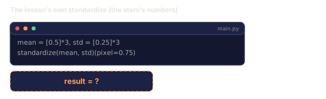
def standardize(mean, std):
    mean = np.array(mean, dtype=np.float32)
    std = np.array(std, dtype=np.float32)
    def _fn(img):
        return (img - mean) / std
    return _fn


def random_hflip(p=0.5):
    def _fn(img):
        if np.random.random() < p:
            return img[:, ::-1, :].copy()
        return img
    return _fn


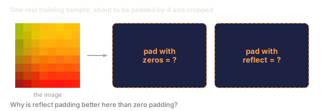
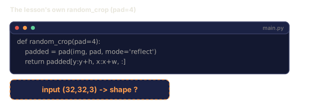
def random_crop(pad=4):
    def _fn(img):
        h, w = img.shape[:2]
        padded = np.pad(img, ((pad, pad), (pad, pad), (0, 0)), mode="reflect")
        y = np.random.randint(0, 2 * pad)
        x = np.random.randint(0, 2 * pad)
        return padded[y:y + h, x:x + w, :]
    return _fn


def compose(*fns):
    def _fn(img):
        for fn in fns:
            img = fn(img)
        return img
    return _fn
Reflect-pad before crop, not zero-pad: a zero-padded crop leaves a hard black border, and the model can learn to key off that border instead of the actual image content.
Step 3: Mixup
Mixes two images and two labels inside the training step. Implemented as a batch transform so it lives next to the forward pass rather than inside the dataset.
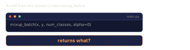
def mixup_batch(x, y, num_classes, alpha=0.2):
    if alpha <= 0:
        return x, torch.nn.functional.one_hot(y, num_classes).float()
    lam = float(np.random.beta(alpha, alpha))
    idx = torch.randperm(x.size(0), device=x.device)
    x_mixed = lam * x + (1 - lam) * x[idx]
    y_onehot = torch.nn.functional.one_hot(y, num_classes).float()
    y_mixed = lam * y_onehot + (1 - lam) * y_onehot[idx]
    return x_mixed, y_mixed


def soft_cross_entropy(logits, soft_targets):
    log_probs = torch.log_softmax(logits, dim=-1)
    return -(soft_targets * log_probs).sum(dim=-1).mean()
soft_cross_entropy is cross-entropy against a soft-label distribution. It reduces to the usual one-hot case when the target is exactly one-hot.
Step 4: The training loop
The complete recipe: one pass over the data, gradients once per batch, scheduler stepped once per epoch.
import torch
import torch.nn as nn
from torch.utils.data import DataLoader
from torch.optim import SGD
from torch.optim.lr_scheduler import CosineAnnealingLR

def train_one_epoch(model, loader, optimizer, device, num_classes, use_mixup=True):
    model.train()
    total, correct, loss_sum = 0, 0, 0.0
    for x, y in loader:
        x, y = x.to(device), y.to(device)
        if use_mixup:
            x_m, y_soft = mixup_batch(x, y, num_classes)
            logits = model(x_m)
            loss = soft_cross_entropy(logits, y_soft)
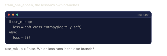
        else:
            logits = model(x)
            loss = nn.functional.cross_entropy(logits, y, label_smoothing=0.1)
        optimizer.zero_grad()
        loss.backward()
        optimizer.step()
        loss_sum += loss.item() * x.size(0)
        total += x.size(0)
        # Training accuracy vs the un-mixed labels `y` is only an approximation
        # when mixup is on (the model saw soft targets, not y). Treat it as a
        # rough progress signal; rely on val accuracy for real performance.
        with torch.no_grad():
            pred = logits.argmax(dim=-1)
            correct += (pred == y).sum().item()
    return loss_sum / total, correct / total


@torch.no_grad()
def evaluate(model, loader, device, num_classes):
    model.eval()
    total, correct = 0, 0
    loss_sum = 0.0
    cm = torch.zeros(num_classes, num_classes, dtype=torch.long)
    for x, y in loader:
        x, y = x.to(device), y.to(device)
        logits = model(x)
        loss = nn.functional.cross_entropy(logits, y)
        pred = logits.argmax(dim=-1)
        for t, p in zip(y.cpu(), pred.cpu()):
            cm[t, p] += 1
        loss_sum += loss.item() * x.size(0)
        total += x.size(0)
        correct += (pred == y).sum().item()
    return loss_sum / total, correct / total, cm
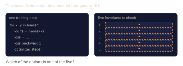
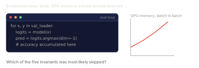
Five invariants you check every time you write a training loop:
model.train()before training,model.eval()before evaluation: this flips dropout and batchnorm behaviour..zero_grad()before.backward()..item()when accumulating metrics so nothing keeps the computation graph alive.@torch.no_grad()during evaluation. It saves memory and time, and it prevents subtle accidents.- Argmax against raw logits, not softmax: same result, one fewer op.
Step 5: Put it together
Use the TinyResNet from the previous lesson, train for a few epochs, evaluate.
from main import synthetic_cifar, ArrayDataset
from main import standardize, random_hflip, random_crop, compose
from main import mixup_batch, soft_cross_entropy
from main import train_one_epoch, evaluate
# TinyResNet comes from the previous lesson (03-cnns-lenet-to-resnet).
# Adjust the import path to wherever you stored the previous lesson's code.
from cnns_lenet_to_resnet import TinyResNet  # example placeholder

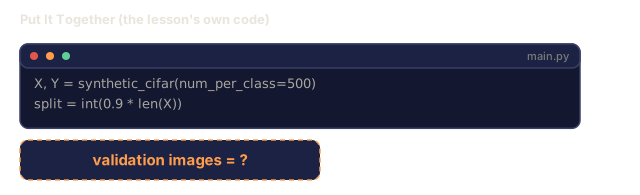
X, Y = synthetic_cifar(num_per_class=500)
split = int(0.9 * len(X))
X_train, Y_train = X[:split], Y[:split]
X_val, Y_val = X[split:], Y[split:]

mean = [0.5, 0.5, 0.5]
std = [0.25, 0.25, 0.25]
train_tf = compose(random_hflip(), random_crop(pad=4), standardize(mean, std))
eval_tf = standardize(mean, std)

train_ds = ArrayDataset(X_train, Y_train, transform=train_tf)
val_ds = ArrayDataset(X_val, Y_val, transform=eval_tf)

train_loader = DataLoader(train_ds, batch_size=128, shuffle=True, num_workers=0)
val_loader = DataLoader(val_ds, batch_size=256, shuffle=False, num_workers=0)

device = "cuda" if torch.cuda.is_available() else "cpu"
model = TinyResNet(num_classes=10).to(device)
optimizer = SGD(model.parameters(), lr=0.1, momentum=0.9, weight_decay=5e-4, nesterov=True)
scheduler = CosineAnnealingLR(optimizer, T_max=10)

for epoch in range(10):
    tr_loss, tr_acc = train_one_epoch(model, train_loader, optimizer, device, 10, use_mixup=True)
    va_loss, va_acc, _ = evaluate(model, val_loader, device, 10)
    scheduler.step()
    print(f"epoch {epoch:2d}  lr {scheduler.get_last_lr()[0]:.4f}  "
          f"train {tr_loss:.3f}/{tr_acc:.3f}  val {va_loss:.3f}/{va_acc:.3f}")
On the synthetic dataset, this gets to near-perfect validation accuracy within five epochs, which is the point: the pipeline is correct, the model can learn what is learnable. Swap the dataset for real CIFAR-10 and the same loop trains to ~90% without changes.
Step 6: Read the confusion matrix
Accuracy alone never tells you where the model is failing. The confusion matrix does.
def print_confusion(cm, labels=None):
    c = cm.shape[0]
    labels = labels or [str(i) for i in range(c)]
    print(f"{'':>6}" + "".join(f"{l:>5}" for l in labels))
    for i in range(c):
        row = cm[i].tolist()
        print(f"{labels[i]:>6}" + "".join(f"{v:>5}" for v in row))
    print()
    tp = cm.diag().float()
    fp = cm.sum(dim=0).float() - tp
    fn = cm.sum(dim=1).float() - tp
    prec = tp / (tp + fp).clamp_min(1)
    rec = tp / (tp + fn).clamp_min(1)
    f1 = 2 * prec * rec / (prec + rec).clamp_min(1e-9)
    for i in range(c):
        print(f"{labels[i]:>6}  prec {prec[i]:.3f}  rec {rec[i]:.3f}  f1 {f1[i]:.3f}")

_, _, cm = evaluate(model, val_loader, device, 10)
print_confusion(cm)
Rows are true classes, columns are predictions. A cluster of off-diagonal counts between classes 3 and 5 means the model confuses those two and gives you a starting point for targeted data collection or a class-specific augmentation.
Use It
torchvision wraps everything above into idiomatic components. For real CIFAR-10 the full pipeline is four lines plus a training loop.
from torchvision.datasets import CIFAR10
from torchvision.transforms import Compose, RandomCrop, RandomHorizontalFlip, ToTensor, Normalize

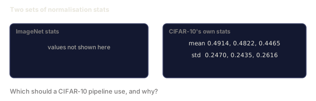
mean = (0.4914, 0.4822, 0.4465)
std = (0.2470, 0.2435, 0.2616)
train_tf = Compose([
    RandomCrop(32, padding=4, padding_mode="reflect"),
    RandomHorizontalFlip(),
    ToTensor(),
    Normalize(mean, std),
])
eval_tf = Compose([ToTensor(), Normalize(mean, std)])

train_ds = CIFAR10(root="./data", train=True,  download=True, transform=train_tf)
val_ds   = CIFAR10(root="./data", train=False, download=True, transform=eval_tf)
Two things to notice: the mean/std are dataset-specific (computed on the CIFAR-10 training set, not ImageNet), and the reflect pad is the community-default crop policy. Copy-pasting ImageNet stats here is a ~1% accuracy leak that nobody catches until someone profiles the model.
Ship It
This lesson produces:
outputs/prompt-classifier-pipeline-auditor.md: a prompt that audits a training script for the five invariants above and surfaces the first violation.outputs/skill-classification-diagnostics.md: a skill that, given a confusion matrix and a list of class names, summarises per-class failures and proposes the single most impactful fix.
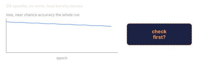
The bug that costs people the most time here isn't mixup or cutmix. It's the double-softmax mistake from the Concept section. I've watched a training run limp along for twenty epochs at close to chance-level accuracy because someone called .softmax() before cross_entropy, and the loss curve still looked like it was doing something. Nothing crashes. Nothing warns you. The only tell is that the number refuses to move, and by the time you notice, you've burned an afternoon second-guessing the architecture instead of the four lines around the loss.
My rule now: the first thing I check in any classifier bug report is what actually goes into the loss function, raw logits or something already squashed. It takes thirty seconds and rules out the single most common silent failure in this whole pipeline.
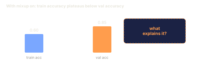
The other one worth calling out is that training-accuracy comment buried in train_one_epoch. When mixup is on, the model trains against soft, blended targets but the code still compares predictions to the original, un-mixed y for a running accuracy number. That number is a rough vibe check, not ground truth. If you ever see train accuracy plateau below val accuracy with mixup on, this is why: don't chase it.
Exercises
- (Easy) Train the same model with and without mixup for five epochs on the synthetic dataset. Plot train and val loss for both. Explain why train loss with mixup is higher yet val accuracy is similar or better.
- (Medium) Implement Cutout (zero out a random 8x8 square in each training image) and run an ablation vs no augmentation, hflip+crop, hflip+crop+cutout, hflip+crop+mixup. Report val accuracy for each.
- (Hard) Build a CIFAR-100 pipeline (100 classes, same input size) and reproduce a ResNet-34 training run to within 1% of published accuracy. Extras: sweep three learning rates and two weight decays, log to a local CSV, produce the final confusion-matrix-top-confusions table.
Key Terms
| Term | What people say | What it actually means |
|---|---|---|
| Logits | "Raw outputs" | The pre-softmax vector of C numbers per image; cross-entropy expects these, not softmaxed values |
| Cross-entropy | "The loss" | Negative log-probability of the correct class; combines log-softmax and NLL in one stable op |
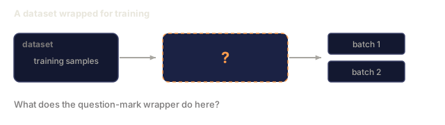
| DataLoader | "The batcher" | Wraps a dataset with shuffling, batching, and (optional) multi-worker loading; gets blamed for half of training bugs |
| Augmentation | "Random transforms" | Any pixel-level transform at training time that preserves the label; teaches invariances the CNN does not have natively |
| Mixup / Cutmix | "Mix two images" | Blend both inputs and labels so the classifier learns smooth interpolations instead of hard boundaries |
| Cutout | "Blank out a patch" | Zero out a random square region of a training image; the label stays unchanged, unlike mixup/cutmix which blend two images' labels |
| Label smoothing | "Softer targets" | Replace one-hot with (1-eps, eps/(C-1), ...); improves calibration and slightly boosts accuracy |
| Top-k accuracy | "Top-5" | The correct class is in the k highest-probability predictions; used on datasets with genuinely ambiguous classes |
| Confusion matrix | "Where errors live" | C x C table where entry (i, j) counts images of true class i predicted as j; diagonal is right, off-diagonal tells you what to fix |
Further Reading
- CS231n: Training Neural Networks — still the clearest tour of the training pipeline at a single page
- Bag of Tricks for Image Classification (He et al., 2019) — every small trick that together adds 3-4% to ResNet accuracy on ImageNet
- mixup: Beyond Empirical Risk Minimization (Zhang et al., 2017) — the original mixup paper; three pages of theory plus convincing experiments
- Why temperature scaling matters (Guo et al., 2017) — the paper that proved modern networks are miscalibrated and fixed it with one scalar parameter
Code
- main.py (python, 216 lines)