Loss Functions
Your network makes a prediction. The ground truth says otherwise. How wrong is it? That number, the loss, is the only thing your optimizer actually minimizes. Pick the wrong one and your model optimizes for the wrong thing entirely.
Learning Objectives
- Implement MSE, binary cross-entropy, categorical cross-entropy, and contrastive loss (InfoNCE) from scratch with their gradients
- Explain why MSE fails for classification by demonstrating the "predict 0.5 for everything" failure mode
- Apply label smoothing to cross-entropy and describe how it prevents overconfident predictions
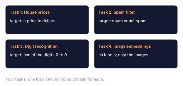
- Choose the correct loss function for regression, binary classification, multi-class classification, and embedding learning tasks
The Problem
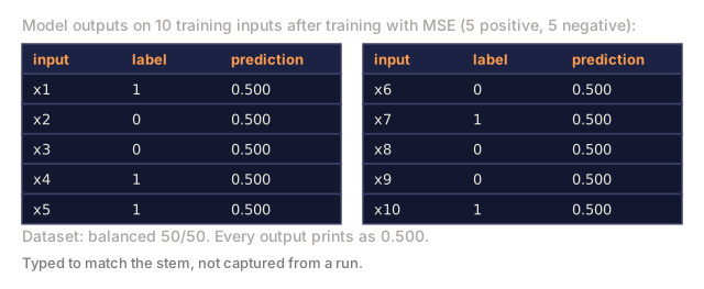
A model minimizing MSE on a classification problem will confidently predict 0.5 for everything. It's minimizing loss. It's also useless.
The loss function is the only thing your model actually optimizes. Not accuracy. Not F1 score. Not whatever metric you report to your manager. The optimizer takes the gradient of the loss function and adjusts weights to make that number smaller. If the loss function doesn't capture what you care about, the model will find the mathematically cheapest way to satisfy it, and that way is almost never what you wanted.
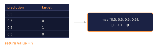
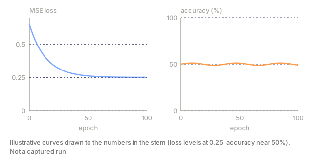
Here is a concrete example. You have a binary classification task. Two classes, 50/50 split. You use MSE as your loss. The model predicts 0.5 for every single input. The average MSE is 0.25, which is the minimum possible without actually learning anything. The model has zero discriminative ability but it has technically minimized your loss function. Switch to cross-entropy and the same model is forced to push predictions toward 0 or 1, because -log(0.5) = 0.693 is a terrible loss, while -log(0.99) = 0.01 rewards confident correct predictions. The choice of loss function is the difference between a model that learns and a model that games the metric.
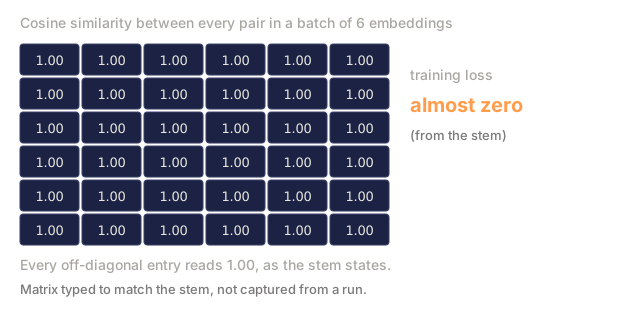
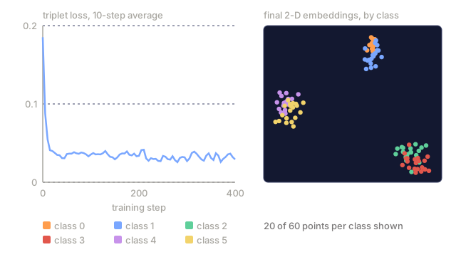
It gets worse. In self-supervised learning, you don't even have labels. Contrastive loss defines the learning signal entirely: what counts as similar, what counts as different, and how hard the model should push them apart. Get contrastive loss wrong and your embeddings collapse to a single point: every input maps to the same vector. Technically zero loss. Completely worthless.
The Concept
Mean Squared Error (MSE)
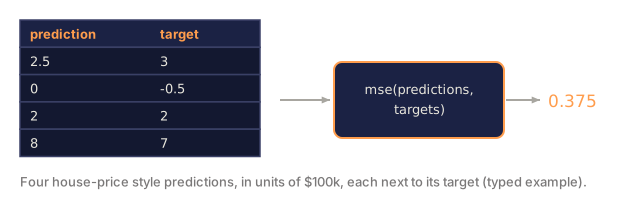
The default for regression. Compute the squared difference between prediction and target, average over all samples.
MSE = (1/n) * sum((y_pred - y_true)^2)
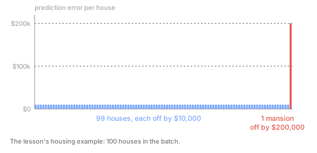
Why squaring matters: it penalizes large errors quadratically. An error of 2 costs 4x as much as an error of 1. An error of 10 costs 100x. This makes MSE sensitive to outliers: a single wildly wrong prediction dominates the loss.
Real numbers: if your model predicts housing prices and is off by $10,000 on most houses but off by $200,000 on one mansion, MSE will aggressively try to fix that one mansion, potentially hurting performance on the other 99 houses.
Analogy: it's like a parking fine that scales with the square of how far over the line you park. Drift two inches over and the fine barely registers. Drift two feet over and the fine doesn't just double, it explodes. MSE prices every miss the same way: distance from the target gets punished quadratically, not linearly.
The gradient of MSE with respect to a prediction is:
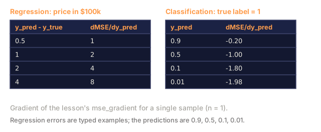
dMSE/dy_pred = (2/n) * (y_pred - y_true)
Linear in the error. Bigger errors get bigger gradients. This is a feature for regression (large errors need large corrections) and a bug for classification (you want to penalize confident wrong answers exponentially, not linearly).
Cross-Entropy Loss
The loss function for classification. It measures the divergence between the predicted probability distribution and the true distribution, an idea rooted in information theory.
Binary Cross-Entropy (BCE):
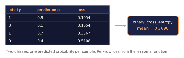
BCE = -(y * log(p) + (1 - y) * log(1 - p))
Where y is the true label (0 or 1) and p is the predicted probability.
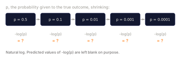
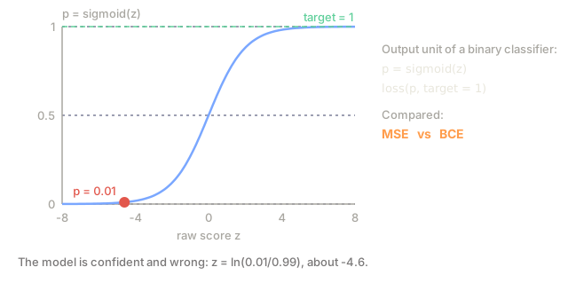
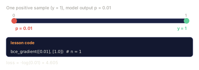
Why -log(p) works: when the true label is 1 and you predict p = 0.99, the loss is -log(0.99) = 0.01. When you predict p = 0.01, the loss is -log(0.01) = 4.6. That 460x difference is why cross-entropy works. It brutally punishes confident wrong predictions while barely penalizing confident correct ones.
Analogy: it's like betting your whole paycheck on a coin flip you were "sure" about, versus hedging a dollar while admitting you're unsure. Confidently wrong costs you far more than modestly wrong, and cross-entropy prices that gap into the loss the same way a bookmaker prices an overconfident bet.
The gradient tells the same story:
dBCE/dp = -(y/p) + (1-y)/(1-p)
When y = 1 and p is near zero, the gradient is -1/p which approaches negative infinity. The model gets an enormous signal to fix its mistake. When p is near 1, the gradient is tiny. Already correct, nothing to fix.
Categorical Cross-Entropy:
For multi-class classification with one-hot encoded targets.
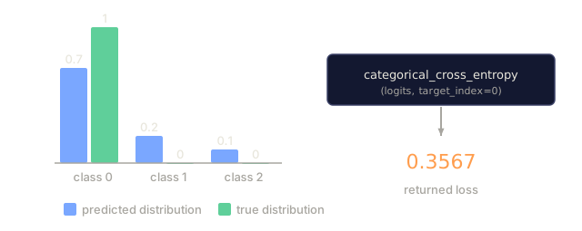
CCE = -sum(y_i * log(p_i))
Only the true class contributes to the loss (because all other y_i are zero). If there are 10 classes and the correct class gets probability 0.1 (random guessing), the loss is -log(0.1) = 2.3. If the correct class gets probability 0.9, the loss is -log(0.9) = 0.105. The model learns to concentrate probability mass on the right answer.
Why MSE Fails for Classification

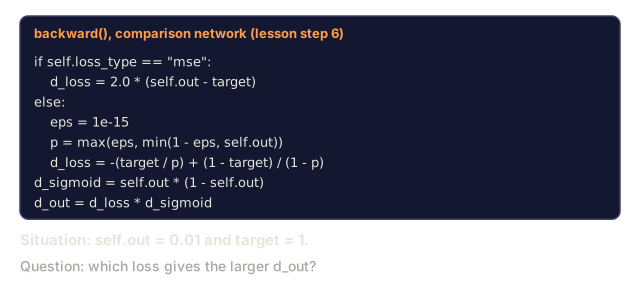
MSE gradients flatten when predictions are near 0 or 1 (due to sigmoid saturation). Cross-entropy gradients compensate for this: the -log cancels the sigmoid's flat regions, giving strong gradients exactly where they are needed most.
Label Smoothing
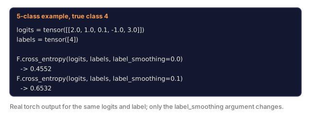
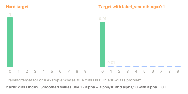
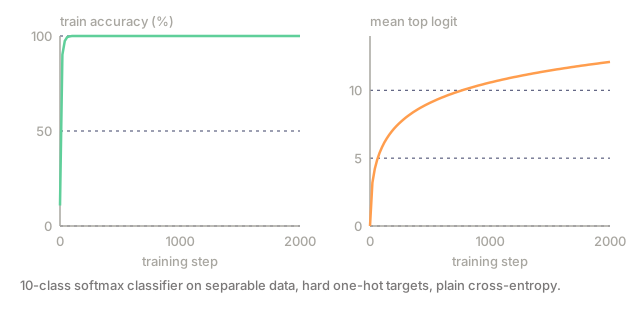
Label smoothing softens hard 0/1 targets instead of forcing the model to match them exactly. Standard one-hot labels say "this is 100% class 3 and 0% everything else," which is a strong claim:
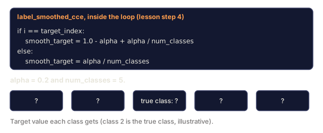
smooth_label = (1 - alpha) * one_hot + alpha / num_classes
With alpha = 0.1 and 10 classes: instead of [0, 0, 1, 0, ...], the target becomes [0.01, 0.01, 0.91, 0.01, ...]. The model targets 0.91 instead of 1.0.
Why this works: a model trying to output exactly 1.0 through a softmax needs to push logits to infinity. This causes overconfidence, hurts generalization, and makes the model brittle to distribution shift. Label smoothing caps the target at 0.9 (with alpha=0.1), keeping logits in a reasonable range. GPT and most modern models use label smoothing or its equivalent.
Contrastive Loss
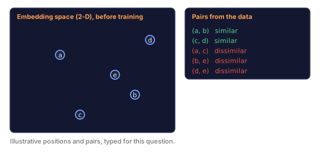
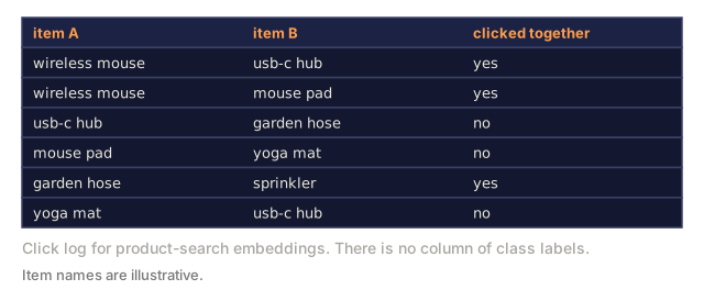
Contrastive loss learns representations without labels: it pulls similar pairs of inputs together in embedding space and pushes dissimilar pairs apart. No classes, no ground truth, just pairs and the question of whether they're similar or different.
SimCLR-style contrastive loss (NT-Xent / InfoNCE):
Take one image. Create two augmented views of it (crop, rotate, color jitter). These are the "positive pair": they should have similar embeddings. Every other image in the batch forms a "negative pair": they should have different embeddings.
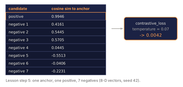
L = -log(exp(sim(z_i, z_j) / tau) / sum(exp(sim(z_i, z_k) / tau)))
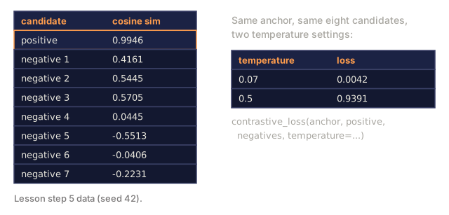
Where sim() is cosine similarity, z_i and z_j are the positive pair, the sum is over all negatives, and tau (temperature) controls how sharp the distribution is. Lower temperature = harder negatives = more aggressive separation.
Real numbers: batch size 256 means 255 negatives per positive pair. Temperature tau = 0.07 (SimCLR default). The loss looks like a softmax over similarities: it wants the positive pair's similarity to be highest among all 256 options.
Analogy: it's like a police lineup. Pull the true match tight against the witness's memory while every other face in the lineup gets pushed further away, and the more suspects standing in that lineup, the sharper the match has to be for the model to still pick the right one.
Triplet Loss:
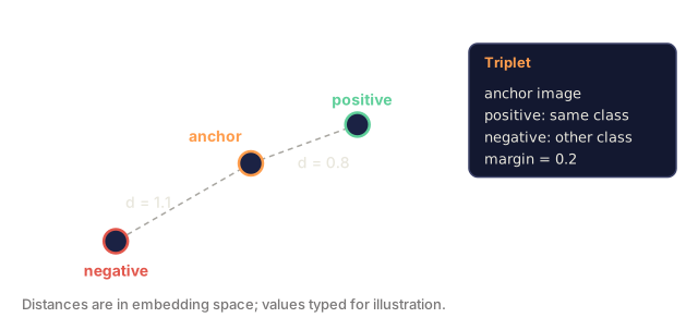
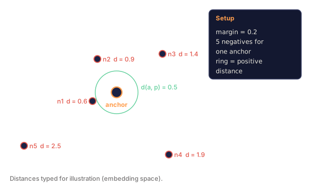
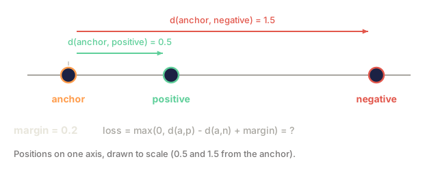
Takes three inputs: anchor, positive (same class), negative (different class).
L = max(0, d(anchor, positive) - d(anchor, negative) + margin)
The margin (typically 0.2-1.0) enforces a minimum gap between positive and negative distances. If the negative is already far enough away, the loss is zero: no gradient, no update. This makes training efficient but requires careful triplet mining (choosing hard negatives that are close to the anchor).
Focal Loss
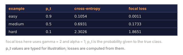
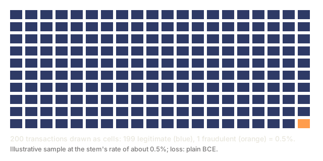
Focal loss down-weights easy examples so training focuses on the hard ones. That's what makes it the fix for imbalanced datasets, where standard cross-entropy treats every correctly classified example equally.
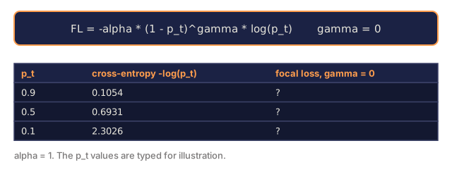
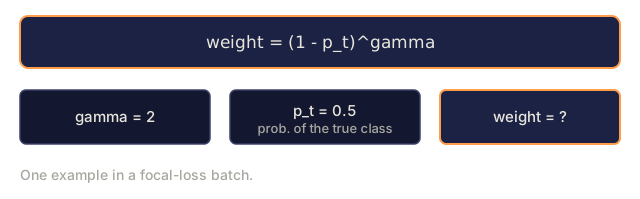
FL = -alpha * (1 - p_t)^gamma * log(p_t)
Where p_t is the predicted probability of the true class and gamma controls the focusing. With gamma = 0, this is standard cross-entropy. With gamma = 2 (the default):
- Easy example (p_t = 0.9): weight = (0.1)^2 = 0.01. Effectively ignored.
- Hard example (p_t = 0.1): weight = (0.9)^2 = 0.81. Full gradient signal.
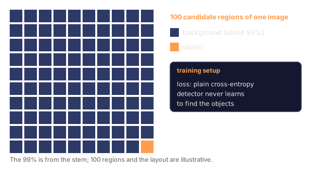
Focal loss was introduced by Lin et al. for object detection, where 99% of candidate regions are background (easy negatives). Without focal loss, the model drowns in easy background examples and never learns to detect objects. With it, the model focuses its capacity on the hard, ambiguous cases that matter.
Loss Function Decision Tree

Loss Landscape

Build It
Step 1: MSE and Its Gradient
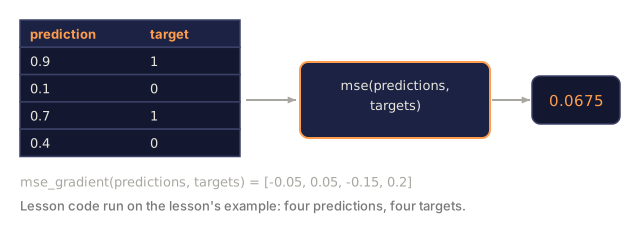
def mse(predictions, targets):
    n = len(predictions)
    total = 0.0
    for p, t in zip(predictions, targets):
        total += (p - t) ** 2
    return total / n

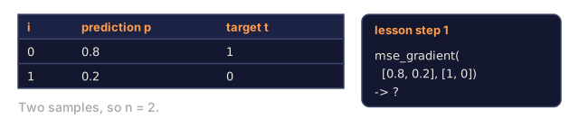
def mse_gradient(predictions, targets):
    n = len(predictions)
    grads = []
    for p, t in zip(predictions, targets):
        grads.append(2.0 * (p - t) / n)
    return grads
Step 2: Binary Cross-Entropy
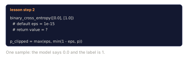
The log(0) problem is real. If the model predicts exactly 0 for a positive example, log(0) = negative infinity. Clipping prevents this.
import math

def binary_cross_entropy(predictions, targets, eps=1e-15):
    n = len(predictions)
    total = 0.0
    for p, t in zip(predictions, targets):
        p_clipped = max(eps, min(1 - eps, p))
        total += -(t * math.log(p_clipped) + (1 - t) * math.log(1 - p_clipped))
    return total / n

def bce_gradient(predictions, targets, eps=1e-15):
    grads = []
    for p, t in zip(predictions, targets):
        p_clipped = max(eps, min(1 - eps, p))
        grads.append(-(t / p_clipped) + (1 - t) / (1 - p_clipped))
    return grads
Step 3: Categorical Cross-Entropy with Softmax
Softmax converts raw logits to probabilities. Then we compute the cross-entropy against one-hot targets.
def softmax(logits):
    max_val = max(logits)
    exps = [math.exp(x - max_val) for x in logits]
    total = sum(exps)
    return [e / total for e in exps]

def categorical_cross_entropy(logits, target_index, eps=1e-15):
    probs = softmax(logits)
    p = max(eps, probs[target_index])
    return -math.log(p)

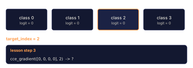
def cce_gradient(logits, target_index):
    probs = softmax(logits)
    grads = list(probs)
    grads[target_index] -= 1.0
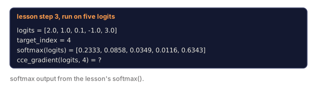
    return grads
The gradient of softmax + cross-entropy simplifies beautifully: it's just (predicted probability - 1) for the true class, and (predicted probability) for all other classes. This elegant simplification is not a coincidence: it's why softmax and cross-entropy are paired.
Step 4: Label Smoothing
def label_smoothed_cce(logits, target_index, num_classes, alpha=0.1, eps=1e-15):
    probs = softmax(logits)
    loss = 0.0
    for i in range(num_classes):
        if i == target_index:
            smooth_target = 1.0 - alpha + alpha / num_classes
        else:
            smooth_target = alpha / num_classes
        p = max(eps, probs[i])
        loss += -smooth_target * math.log(p)
    return loss
Step 5: Contrastive Loss (Simplified InfoNCE)
def cosine_similarity(a, b):
    dot = sum(x * y for x, y in zip(a, b))
    norm_a = math.sqrt(sum(x * x for x in a))
    norm_b = math.sqrt(sum(x * x for x in b))
    if norm_a < 1e-10 or norm_b < 1e-10:
        return 0.0
    return dot / (norm_a * norm_b)

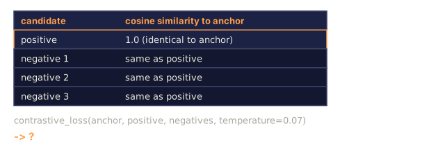
def contrastive_loss(anchor, positive, negatives, temperature=0.07):
    sim_pos = cosine_similarity(anchor, positive) / temperature
    sim_negs = [cosine_similarity(anchor, neg) / temperature for neg in negatives]

    max_sim = max(sim_pos, max(sim_negs)) if sim_negs else sim_pos
    exp_pos = math.exp(sim_pos - max_sim)
    exp_negs = [math.exp(s - max_sim) for s in sim_negs]
    total_exp = exp_pos + sum(exp_negs)

    return -math.log(max(1e-15, exp_pos / total_exp))
Step 6: MSE vs Cross-Entropy on Classification
Train the same network from lesson 04 (circle dataset) with both loss functions. Watch cross-entropy converge faster.
import random

def sigmoid(x):
    x = max(-500, min(500, x))
    return 1.0 / (1.0 + math.exp(-x))

def make_circle_data(n=200, seed=42):
    random.seed(seed)
    data = []
    for _ in range(n):
        x = random.uniform(-2, 2)
        y = random.uniform(-2, 2)
        label = 1.0 if x * x + y * y < 1.5 else 0.0
        data.append(([x, y], label))
    return data


class LossComparisonNetwork:
    def __init__(self, loss_type="bce", hidden_size=8, lr=0.1):
        random.seed(0)
        self.loss_type = loss_type
        self.lr = lr
        self.hidden_size = hidden_size

        self.w1 = [[random.gauss(0, 0.5) for _ in range(2)] for _ in range(hidden_size)]
        self.b1 = [0.0] * hidden_size
        self.w2 = [random.gauss(0, 0.5) for _ in range(hidden_size)]
        self.b2 = 0.0

    def forward(self, x):
        self.x = x
        self.z1 = []
        self.h = []
        for i in range(self.hidden_size):
            z = self.w1[i][0] * x[0] + self.w1[i][1] * x[1] + self.b1[i]
            self.z1.append(z)
            self.h.append(max(0.0, z))

        self.z2 = sum(self.w2[i] * self.h[i] for i in range(self.hidden_size)) + self.b2
        self.out = sigmoid(self.z2)
        return self.out

    def backward(self, target):
        if self.loss_type == "mse":
            d_loss = 2.0 * (self.out - target)
        else:
            eps = 1e-15
            p = max(eps, min(1 - eps, self.out))
            d_loss = -(target / p) + (1 - target) / (1 - p)

        d_sigmoid = self.out * (1 - self.out)
        d_out = d_loss * d_sigmoid

        for i in range(self.hidden_size):
            d_relu = 1.0 if self.z1[i] > 0 else 0.0
            d_h = d_out * self.w2[i] * d_relu
            self.w2[i] -= self.lr * d_out * self.h[i]
            for j in range(2):
                self.w1[i][j] -= self.lr * d_h * self.x[j]
            self.b1[i] -= self.lr * d_h
        self.b2 -= self.lr * d_out

    def compute_loss(self, pred, target):
        if self.loss_type == "mse":
            return (pred - target) ** 2
        else:
            eps = 1e-15
            p = max(eps, min(1 - eps, pred))
            return -(target * math.log(p) + (1 - target) * math.log(1 - p))

    def train(self, data, epochs=200):
        losses = []
        for epoch in range(epochs):
            total_loss = 0.0
            correct = 0
            for x, y in data:
                pred = self.forward(x)
                self.backward(y)
                total_loss += self.compute_loss(pred, y)
                if (pred >= 0.5) == (y >= 0.5):
                    correct += 1
            avg_loss = total_loss / len(data)
            accuracy = correct / len(data) * 100
            losses.append((avg_loss, accuracy))
            if epoch % 50 == 0 or epoch == epochs - 1:
                print(f"    Epoch {epoch:3d}: loss={avg_loss:.4f}, accuracy={accuracy:.1f}%")
        return losses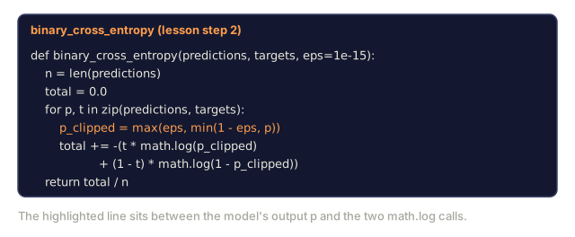
Use It
PyTorch provides all standard loss functions with numerical stability built in:
import torch
import torch.nn as nn
import torch.nn.functional as F

predictions = torch.tensor([0.9, 0.1, 0.7], requires_grad=True)
targets = torch.tensor([1.0, 0.0, 1.0])

mse_loss = F.mse_loss(predictions, targets)
bce_loss = F.binary_cross_entropy(predictions, targets)

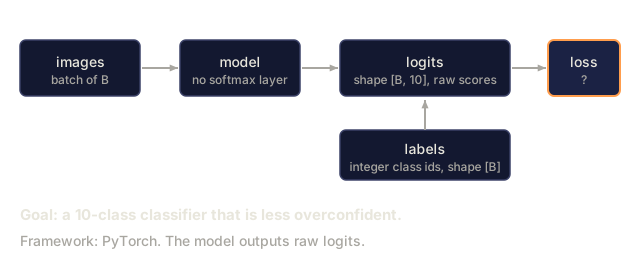
logits = torch.randn(4, 10)
labels = torch.tensor([3, 7, 1, 9])
ce_loss = F.cross_entropy(logits, labels)
ce_smooth = F.cross_entropy(logits, labels, label_smoothing=0.1)
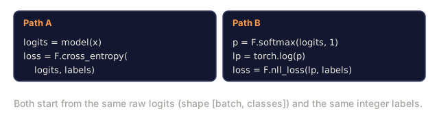
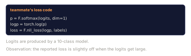
Use F.cross_entropy (not F.nll_loss plus manual softmax). It combines log-softmax and negative log-likelihood in one numerically stable operation. Applying softmax separately then taking the log is less stable: you lose precision in the subtraction of large exponentials.
For contrastive learning, most teams use custom implementations or libraries like lightly or pytorch-metric-learning. The core loop is always the same: compute pairwise similarities, create the softmax over positives and negatives, backpropagate.
Ship It
This lesson produces:
outputs/prompt-loss-function-selector.md, a reusable prompt for choosing the right loss functionoutputs/prompt-loss-debugger.md, a diagnostic prompt for when your loss curve looks wrong
The loss curve lies to you in one specific, recurring way: it goes down smoothly while the model learns nothing useful. I've hit this exact failure twice. Once with MSE on a classification task, where the number looked great because the model had converged to predicting 0.5 for everything. Once with a contrastive setup where the embeddings quietly collapsed to a single point: cosine similarity between every pair in the batch sat at 1.0, and the loss was practically zero. Both times the fix was the same. Stop staring at the loss number and look at what the model actually outputs. Print ten predictions. Check the variance of your embeddings. Do that before you trust the curve. A falling loss curve proves the optimizer did its job on whatever function you handed it. It doesn't prove that function is the one you meant to write.
Exercises
-
Implement Huber loss (smooth L1 loss), which is MSE for small errors and MAE for large errors. Train a regression network predicting y = sin(x) with MSE vs Huber when 5% of training targets have random noise added (outliers). Compare final test error.
-
Add focal loss to the binary classification training loop. Create an imbalanced dataset (90% class 0, 10% class 1). Compare standard BCE vs focal loss (gamma=2) on the minority class recall after 200 epochs.
-
Implement triplet loss with semi-hard negative mining. Generate 2D embedding data for 5 classes. For each anchor, find the hardest negative that is still farther than the positive (semi-hard). Compare convergence to random triplet selection.
-
Run the MSE vs cross-entropy comparison but track gradient magnitudes at each layer during training. Plot the average gradient norm per epoch. Verify that cross-entropy produces larger gradients in early epochs when the model is most uncertain.
-
Implement KL divergence loss and verify that minimizing KL(true || predicted) gives the same gradients as cross-entropy when the true distribution is one-hot. Then try soft targets (like knowledge distillation) where the "true" distribution comes from a teacher model's softmax output.
Key Terms
| Term | What people say | What it actually means |
|---|---|---|
| Loss function | "How wrong the model is" | A differentiable function mapping predictions and targets to a scalar that the optimizer minimizes |
| MSE | "Average squared error" | Mean of squared differences between predictions and targets; penalizes large errors quadratically |
| Cross-entropy | "The classification loss" | Measures divergence between predicted probability distribution and true distribution using -log(p) |
| Binary cross-entropy | "BCE" | Cross-entropy for two classes: -(y*log(p) + (1-y)*log(1-p)) |
| Label smoothing | "Softening the targets" | Replacing hard 0/1 targets with soft values (e.g., 0.1/0.9) to prevent overconfidence and improve generalization |
| Contrastive loss | "Pull together, push apart" | A loss that learns representations by making similar pairs close and dissimilar pairs far in embedding space |
| InfoNCE | "The CLIP/SimCLR loss" | Normalized temperature-scaled cross-entropy over similarity scores; treats contrastive learning as classification |
| Focal loss | "The imbalanced data fix" | Cross-entropy weighted by (1-p_t)^gamma to down-weight easy examples and focus on hard ones |
| Triplet loss | "Anchor-positive-negative" | Pushes anchor closer to positive than negative by at least a margin in embedding space |
| Temperature | "Sharpness knob" | A scalar divisor on logits/similarities that controls how peaked the resulting distribution is; lower = sharper |
Further Reading
- Lin et al., "Focal Loss for Dense Object Detection" (2017) — introduced focal loss for handling extreme class imbalance in object detection (RetinaNet)
- Chen et al., "A Simple Framework for Contrastive Learning of Visual Representations" (SimCLR, 2020) — defined the modern contrastive learning pipeline with NT-Xent loss
- Szegedy et al., "Rethinking the Inception Architecture" (2016) — introduced label smoothing as a regularization technique, now standard in most large models
- Hinton et al., "Distilling the Knowledge in a Neural Network" (2015) — knowledge distillation using soft targets and KL divergence, foundational for model compression