Optimizers
Gradient descent points you in the right direction. It has no opinion on how far to step, or whether that step should change as training goes on. SGD is a compass. Adam is GPS with live traffic data.
Learning Objectives
- Implement SGD, SGD with momentum, Adam, and AdamW optimizers from scratch in Python
- Explain how Adam's bias correction compensates for zero-initialized moment estimates in early training steps
- Demonstrate why AdamW produces better generalization than Adam with L2 regularization on the same task
- Select the appropriate optimizer and default hyperparameters for transformers, CNNs, GANs, and fine-tuning
The Problem
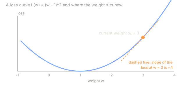
You computed the gradients. Weight #4,721 needs to decrease by 0.003 to reduce the loss. But 0.003 in what units, scaled by what, and should you move by that same amount on step 1 as on step 1,000?
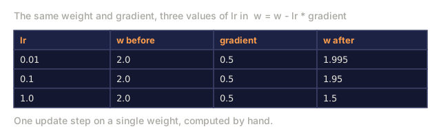
Vanilla gradient descent applies the same learning rate to every parameter on every step: w = w - lr * gradient. That single choice creates three problems that make training painful in practice.
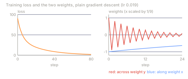
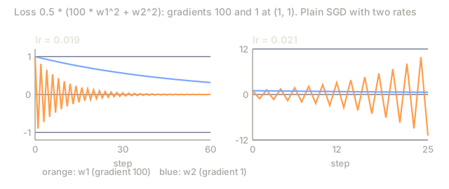
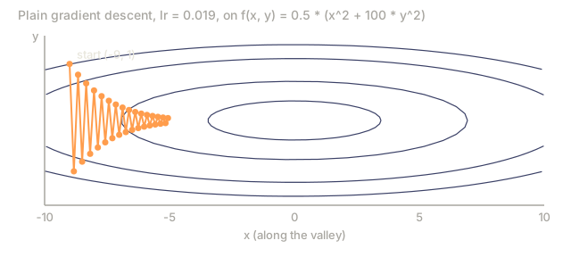
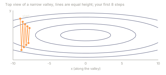
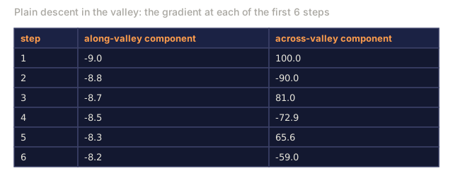
First, oscillation. The loss landscape is rarely a smooth bowl; it's more often a long, narrow valley, where the gradient points across the valley (steep direction) instead of along it (shallow direction). Gradient descent bounces back and forth across the narrow dimension while it barely creeps along the useful one. You've seen the result: loss drops fast, then plateaus, not because the model converged but because it's oscillating.
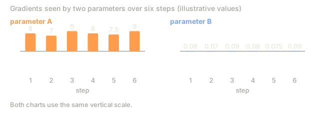
Second, one learning rate for every parameter is wrong. Some weights need large updates because they're still early and underfitting. Others need tiny updates because they're already close to their optimal value. A rate that works for the former destroys the latter, and vice versa.
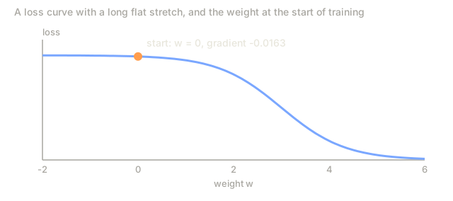
Third, saddle points. In high dimensions, the loss landscape has vast flat regions where the gradient is near zero, and vanilla SGD crawls through them at the speed of that near-zero gradient. The model looks stuck. It isn't: there's useful descent waiting on the other side of that flat region, but SGD has no mechanism to push through and find it.
Adam solves all three at once. It keeps two running averages per parameter: the mean gradient (momentum, which handles oscillation) and the mean squared gradient (adaptive rate, which handles the different scales). Add bias correction for the first few steps and you get a single optimizer that works on 80% of problems with default hyperparameters. Build it from scratch, which is exactly what this lesson does, and you'll know precisely when and why it fails on the other 20%.
The Concept
Stochastic Gradient Descent (SGD)
The simplest optimizer. Compute the gradient on a mini-batch and step in the opposite direction.
w = w - lr * gradient
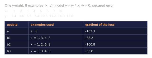
The "stochastic" part means you estimate the gradient from a random subset (mini-batch) rather than the full dataset. That randomness helps the optimizer escape sharp local minima, but it's also the source of the oscillation problem above.
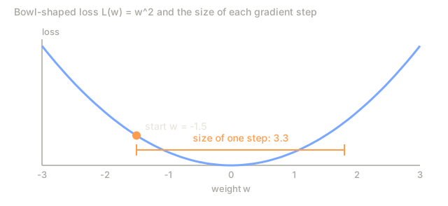
Learning rate is the only knob. Too high: the loss diverges. Too low: training takes forever. The optimal value depends on the architecture, the data, the batch size, and the current stage of training. For vanilla SGD on modern networks, typical values range from 0.01 to 0.1. But even within a single training run, the ideal learning rate changes.
Momentum
Instead of stepping by the gradient alone, you maintain a velocity that accumulates past gradients. Call it the ball-rolling-downhill analogy if you want; overused, but accurate here.
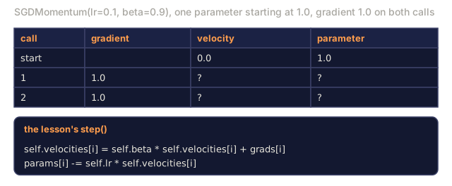
m_t = beta * m_{t-1} + gradient
w = w - lr * m_t
Beta (typically 0.9) controls how much history to keep. With beta = 0.9, the momentum is roughly the average of the last 10 gradients (1 / (1 - 0.9) = 10).
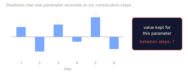
Why this fixes oscillation: gradients that point in the same direction accumulate. Gradients that flip direction cancel out. In that narrow valley, the "across" component flips sign each step and gets dampened. The "along" component stays consistent and gets amplified. The result is smooth acceleration in the useful direction.
Real numbers: SGD alone on a badly conditioned loss landscape might take 10,000 steps. SGD with momentum (beta=0.9) typically takes 3,000-5,000 steps on the same problem. The speedup is not marginal.
RMSProp
The first per-parameter adaptive learning rate method that actually worked. Proposed by Hinton in a Coursera lecture (never formally published).
s_t = beta * s_{t-1} + (1 - beta) * gradient^2
w = w - lr * gradient / (sqrt(s_t) + epsilon)
s_t tracks the running average of squared gradients. Parameters with consistently large gradients get divided by a large number (smaller effective learning rate). Parameters with small gradients get divided by a small number (larger effective learning rate).
This solves the "one learning rate for all parameters" problem. A weight that's already been getting large updates is probably near its target: slow it down. A weight that's been getting tiny updates might be undertrained: speed it up.
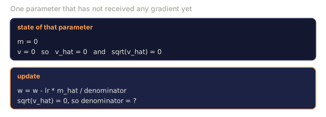
Epsilon (typically 1e-8) prevents division by zero when a parameter hasn't been updated.
Adam: Momentum + RMSProp
Adam combines both ideas. It maintains two exponential moving averages per parameter:
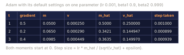
m_t = beta1 * m_{t-1} + (1 - beta1) * gradient        (first moment: mean)
v_t = beta2 * v_{t-1} + (1 - beta2) * gradient^2       (second moment: variance)
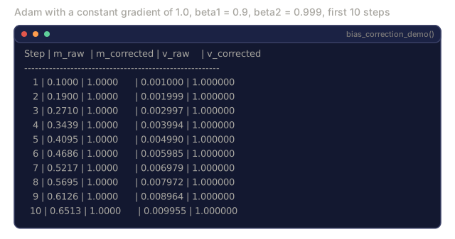
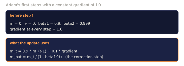
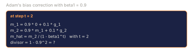
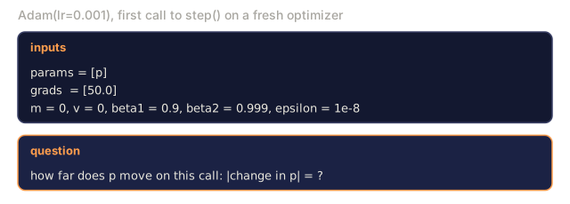
Bias correction is the key detail most explanations skip. At step 1, m_1 = (1 - beta1) * gradient. With beta1 = 0.9, that's 0.1 * gradient: ten times too small. The moving average hasn't warmed up yet. Bias correction compensates:
m_hat = m_t / (1 - beta1^t)
v_hat = v_t / (1 - beta2^t)
At step 1 with beta1 = 0.9: m_hat = m_1 / (1 - 0.9) = m_1 / 0.1 = the actual gradient. At step 100: (1 - 0.9^100) is approximately 1.0, so the correction vanishes. Bias correction matters for the first ~10 steps and is irrelevant after ~50.
The update:
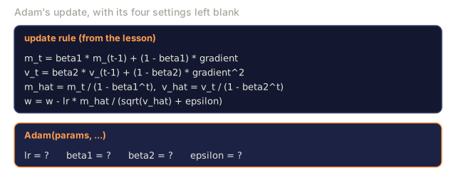
w = w - lr * m_hat / (sqrt(v_hat) + epsilon)
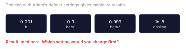
Adam defaults: lr = 0.001, beta1 = 0.9, beta2 = 0.999, epsilon = 1e-8. These defaults work for 80% of problems. When they don't, change lr first. Then beta2. Almost never change beta1 or epsilon.
AdamW: Weight Decay Done Right
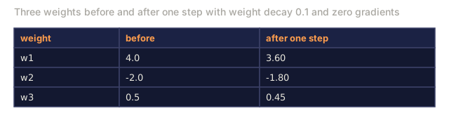
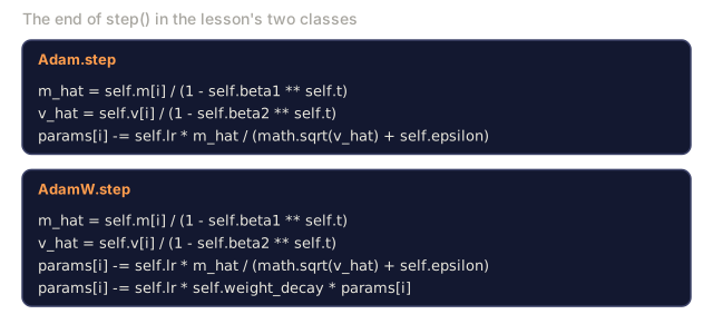
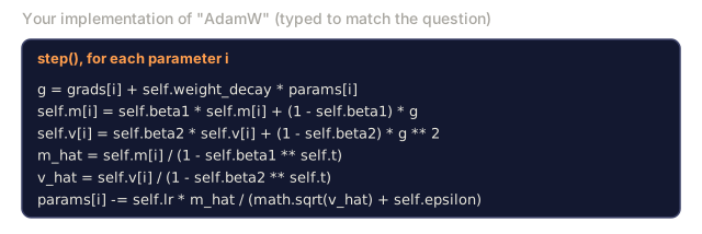
AdamW is Adam with one change: weight decay gets applied straight to the weights, after the Adam update, instead of folded into the gradient through L2 regularization. Here's why that distinction matters.
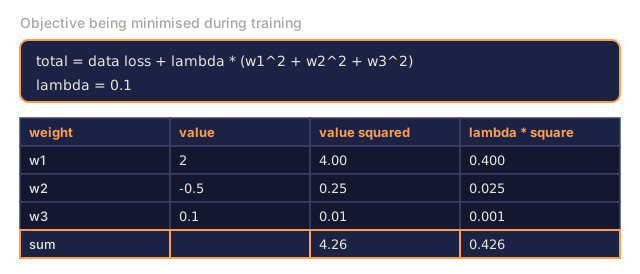
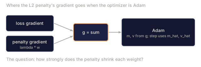
L2 regularization adds lambda * w^2 to the loss. In vanilla SGD, this is equivalent to weight decay (subtracting lambda * w from the weight at each step). In Adam, this equivalence breaks.
The Loshchilov & Hutter insight: when you add L2 to the loss and Adam processes the gradient, the adaptive learning rate scales the regularization term too. Parameters with large gradient variance get less regularization. Parameters with small variance get more. That's the opposite of what you want: uniform regularization regardless of the gradient statistics.
AdamW fixes this by applying weight decay directly to the weights, after the Adam update:
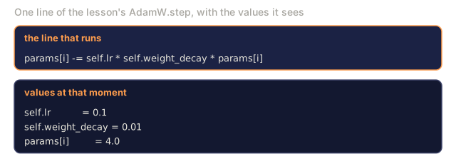
w = w - lr * m_hat / (sqrt(v_hat) + epsilon) - lr * lambda * w
The weight decay term (lr * lambda * w) is not scaled by Adam's adaptive factor. Every parameter gets the same proportional shrinkage.
This seems like a minor detail. It's not. AdamW converges to better solutions than Adam + L2 regularization on virtually every task. It's the default optimizer in PyTorch for training transformers, diffusion models, and most modern architectures. BERT, GPT, LLaMA, Stable Diffusion: all trained with AdamW.
Learning Rate: The Most Important Hyperparameter

If you tune one hyperparameter, tune the learning rate. A 10x change in learning rate matters more than any architectural decision you'll make. Common defaults:
- SGD: lr = 0.01 to 0.1
- Adam/AdamW: lr = 1e-4 to 3e-4
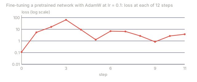
- Fine-tuning pretrained models: lr = 1e-5 to 5e-5
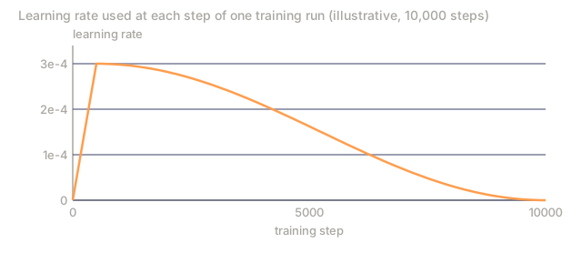
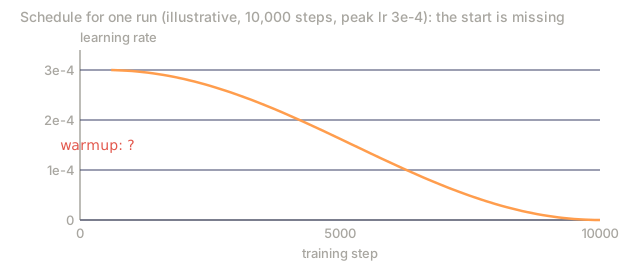
- Learning rate warmup: linear ramp over first 1-10% of steps
Optimizer Comparison

When Each Optimizer Wins

Build It
Step 1: Vanilla SGD
class SGD:
    def __init__(self, lr=0.01):
        self.lr = lr

    def step(self, params, grads):
        for i in range(len(params)):
            params[i] -= self.lr * grads[i]
Step 2: SGD with Momentum
class SGDMomentum:
    def __init__(self, lr=0.01, beta=0.9):
        self.lr = lr
        self.beta = beta
        self.velocities = None

    def step(self, params, grads):
        if self.velocities is None:
            self.velocities = [0.0] * len(params)
        for i in range(len(params)):
            self.velocities[i] = self.beta * self.velocities[i] + grads[i]
            params[i] -= self.lr * self.velocities[i]
Step 3: Adam
import math

class Adam:
    def __init__(self, lr=0.001, beta1=0.9, beta2=0.999, epsilon=1e-8):
        self.lr = lr
        self.beta1 = beta1
        self.beta2 = beta2
        self.epsilon = epsilon
        self.m = None
        self.v = None
        self.t = 0

    def step(self, params, grads):
        if self.m is None:
            self.m = [0.0] * len(params)
            self.v = [0.0] * len(params)

        self.t += 1

        for i in range(len(params)):
            self.m[i] = self.beta1 * self.m[i] + (1 - self.beta1) * grads[i]
            self.v[i] = self.beta2 * self.v[i] + (1 - self.beta2) * grads[i] ** 2

            m_hat = self.m[i] / (1 - self.beta1 ** self.t)
            v_hat = self.v[i] / (1 - self.beta2 ** self.t)

            params[i] -= self.lr * m_hat / (math.sqrt(v_hat) + self.epsilon)
Step 4: AdamW
class AdamW:
    def __init__(self, lr=0.001, beta1=0.9, beta2=0.999, epsilon=1e-8, weight_decay=0.01):
        self.lr = lr
        self.beta1 = beta1
        self.beta2 = beta2
        self.epsilon = epsilon
        self.weight_decay = weight_decay
        self.m = None
        self.v = None
        self.t = 0

    def step(self, params, grads):
        if self.m is None:
            self.m = [0.0] * len(params)
            self.v = [0.0] * len(params)

        self.t += 1

        for i in range(len(params)):
            self.m[i] = self.beta1 * self.m[i] + (1 - self.beta1) * grads[i]
            self.v[i] = self.beta2 * self.v[i] + (1 - self.beta2) * grads[i] ** 2

            m_hat = self.m[i] / (1 - self.beta1 ** self.t)
            v_hat = self.v[i] / (1 - self.beta2 ** self.t)

            params[i] -= self.lr * m_hat / (math.sqrt(v_hat) + self.epsilon)
            params[i] -= self.lr * self.weight_decay * params[i]
Step 5: Training Comparison
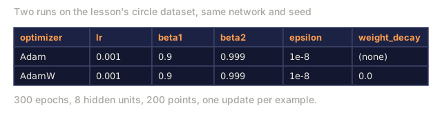
Train the same two-layer network on the circle dataset from lesson 05 with all four optimizers. Compare convergence.
import random

def sigmoid(x):
    x = max(-500, min(500, x))
    return 1.0 / (1.0 + math.exp(-x))

def make_circle_data(n=200, seed=42):
    random.seed(seed)
    data = []
    for _ in range(n):
        x = random.uniform(-2, 2)
        y = random.uniform(-2, 2)
        label = 1.0 if x * x + y * y < 1.5 else 0.0
        data.append(([x, y], label))
    return data


class OptimizerTestNetwork:
    def __init__(self, optimizer, hidden_size=8):
        random.seed(0)
        self.hidden_size = hidden_size
        self.optimizer = optimizer

        self.w1 = [[random.gauss(0, 0.5) for _ in range(2)] for _ in range(hidden_size)]
        self.b1 = [0.0] * hidden_size
        self.w2 = [random.gauss(0, 0.5) for _ in range(hidden_size)]
        self.b2 = 0.0

    def get_params(self):
        params = []
        for row in self.w1:
            params.extend(row)
        params.extend(self.b1)
        params.extend(self.w2)
        params.append(self.b2)
        return params

    def set_params(self, params):
        idx = 0
        for i in range(self.hidden_size):
            for j in range(2):
                self.w1[i][j] = params[idx]
                idx += 1
        for i in range(self.hidden_size):
            self.b1[i] = params[idx]
            idx += 1
        for i in range(self.hidden_size):
            self.w2[i] = params[idx]
            idx += 1
        self.b2 = params[idx]

    def forward(self, x):
        self.x = x
        self.z1 = []
        self.h = []
        for i in range(self.hidden_size):
            z = self.w1[i][0] * x[0] + self.w1[i][1] * x[1] + self.b1[i]
            self.z1.append(z)
            self.h.append(max(0.0, z))

        self.z2 = sum(self.w2[i] * self.h[i] for i in range(self.hidden_size)) + self.b2
        self.out = sigmoid(self.z2)
        return self.out

    def compute_grads(self, target):
        eps = 1e-15
        p = max(eps, min(1 - eps, self.out))
        d_loss = -(target / p) + (1 - target) / (1 - p)
        d_sigmoid = self.out * (1 - self.out)
        d_out = d_loss * d_sigmoid

        grads = [0.0] * (self.hidden_size * 2 + self.hidden_size + self.hidden_size + 1)
        idx = 0
        for i in range(self.hidden_size):
            d_relu = 1.0 if self.z1[i] > 0 else 0.0
            d_h = d_out * self.w2[i] * d_relu
            grads[idx] = d_h * self.x[0]
            grads[idx + 1] = d_h * self.x[1]
            idx += 2

        for i in range(self.hidden_size):
            d_relu = 1.0 if self.z1[i] > 0 else 0.0
            grads[idx] = d_out * self.w2[i] * d_relu
            idx += 1

        for i in range(self.hidden_size):
            grads[idx] = d_out * self.h[i]
            idx += 1

        grads[idx] = d_out
        return grads

    def train(self, data, epochs=300):
        losses = []
        for epoch in range(epochs):
            total_loss = 0.0
            correct = 0
            for x, y in data:
                pred = self.forward(x)
                grads = self.compute_grads(y)
                params = self.get_params()
                self.optimizer.step(params, grads)
                self.set_params(params)

                eps = 1e-15
                p = max(eps, min(1 - eps, pred))
                total_loss += -(y * math.log(p) + (1 - y) * math.log(1 - p))
                if (pred >= 0.5) == (y >= 0.5):
                    correct += 1
            avg_loss = total_loss / len(data)
            accuracy = correct / len(data) * 100
            losses.append((avg_loss, accuracy))
            if epoch % 75 == 0 or epoch == epochs - 1:
                print(f"    Epoch {epoch:3d}: loss={avg_loss:.4f}, accuracy={accuracy:.1f}%")
        return losses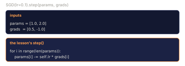
Use It
PyTorch optimizers handle parameter groups, gradient clipping, and learning rate scheduling:
import torch
import torch.optim as optim

model = torch.nn.Sequential(
    torch.nn.Linear(784, 256),
    torch.nn.ReLU(),
    torch.nn.Linear(256, 10),
)

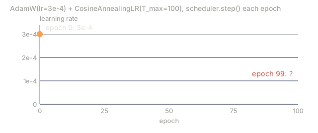
optimizer = optim.AdamW(model.parameters(), lr=3e-4, weight_decay=0.01)

scheduler = optim.lr_scheduler.CosineAnnealingLR(optimizer, T_max=100)

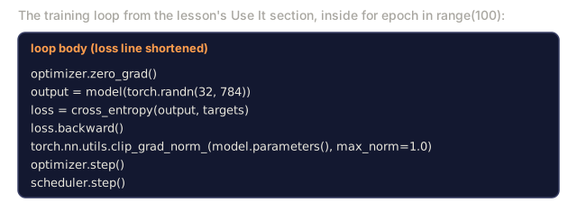
for epoch in range(100):
    optimizer.zero_grad()
    output = model(torch.randn(32, 784))
    loss = torch.nn.functional.cross_entropy(output, torch.randint(0, 10, (32,)))
    loss.backward()
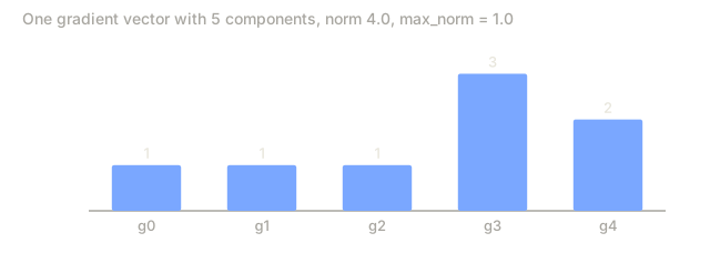
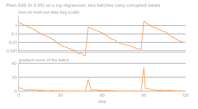
    torch.nn.utils.clip_grad_norm_(model.parameters(), max_norm=1.0)
    optimizer.step()
    scheduler.step()
CosineAnnealingLR glides the learning rate down along a cosine curve toward zero over T_max steps, instead of dropping it in sudden jumps.
The pattern is always: zero_grad, forward, loss, backward, (clip), step, (schedule). Memorize this order. Getting it wrong (e.g., calling scheduler.step() before optimizer.step()) is a common source of subtle bugs.
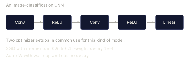
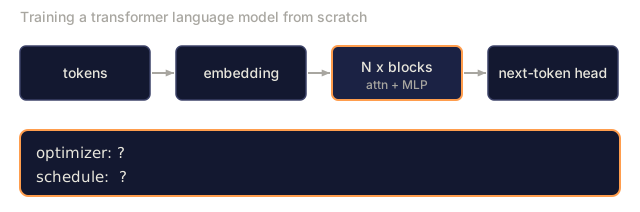
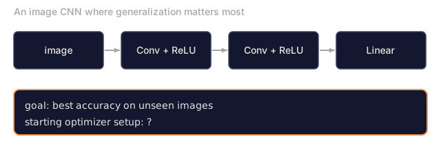
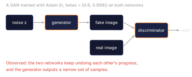
For CNNs, many practitioners still prefer SGD + momentum (lr=0.1, momentum=0.9, weight_decay=1e-4) with a step or cosine schedule. SGD finds flatter minima, which often generalize better. For transformers and LLMs, AdamW with warmup + cosine decay is the universal default. For GANs, drop Adam's beta1 from the default 0.9 to about 0.5: high momentum amplifies the back-and-forth instability between generator and discriminator and pushes training toward mode collapse, a fix that traces back to the DCGAN paper. Some setups go further and give the generator and discriminator separate learning rates entirely (TTUR). Don't fight the consensus without a measured reason.
Ship It
This lesson produces:
outputs/prompt-optimizer-selector.md, a decision prompt for choosing the right optimizer and learning rate for any architecture
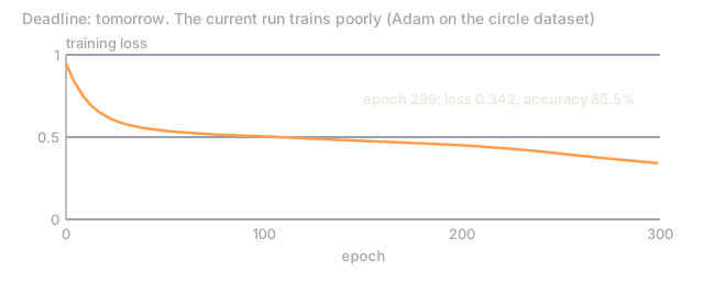
Most online arguments about which optimizer is "best" are really arguments about learning rate that got mislabeled. Swap AdamW for Adam at the same learning rate with weight decay set to zero and you'll barely see a difference; the gap only opens up once weight decay is actually doing something, which in practice is most of the time. If you're short on time before a deadline, don't burn it on an optimizer bake-off. Sweep the learning rate across two or three orders of magnitude on whatever optimizer you already have running. That's the knob that decides whether training works at all, and it's the one people reach for last.
Exercises
-
Implement Nesterov momentum, where you compute the gradient at the "lookahead" position (w - lr * beta * v) instead of the current position. Compare convergence to standard momentum on the circle dataset.
-
Implement a learning rate warmup schedule: linear ramp from 0 to max_lr over the first 10% of training steps, then cosine decay to 0. Train with Adam + warmup vs Adam without warmup. Measure how many epochs it takes to reach 90% accuracy on the circle dataset.
-
Track the effective learning rate for each parameter during Adam training. The effective rate is lr * m_hat / (sqrt(v_hat) + eps). Plot the distribution of effective rates after 10, 50, and 200 steps. Are all parameters being updated at the same speed?
-
Implement gradient clipping (clip by global norm). Set the max gradient norm to 1.0. Train with and without clipping using a high learning rate (lr=0.01 for Adam). Count how many runs diverge (loss goes to NaN) with and without clipping over 10 random seeds.
-
Compare Adam vs AdamW on a network with large weights. Initialize all weights to random values in [-5, 5] (much larger than normal). Train for 200 epochs with weight_decay=0.1. Plot the L2 norm of weights over training for both optimizers. AdamW should show faster weight shrinkage.
Key Terms
| Term | What people say | What it actually means |
|---|---|---|
| Learning rate | "Step size" | The scalar multiplier on the gradient update; the single most impactful hyperparameter in training |
| SGD | "Basic gradient descent" | Stochastic gradient descent: update weights by subtracting lr * gradient, computed on a mini-batch |
| Momentum | "Rolling ball analogy" | Exponential moving average of past gradients; dampens oscillation and accelerates consistent directions |
| RMSProp | "Adaptive learning rate" | Divides each parameter's gradient by the running RMS of its recent gradients; equalizes learning rates |
| Adam | "The default optimizer" | Combines momentum (first moment) and RMSProp (second moment) with bias correction for the initial steps |
| AdamW | "Adam done right" | Adam with decoupled weight decay; applies regularization directly to weights rather than through the gradient |
| Bias correction | "Warmup for running averages" | Dividing by (1 - beta^t) to compensate for the zero-initialization of Adam's moment estimates |
| Weight decay | "Shrink the weights" | Subtracting a fraction of the weight value at each step; a regularizer that penalizes large weights |
| Learning rate schedule | "Changing lr over time" | A function that adjusts the learning rate during training; warmup + cosine decay is the modern default |
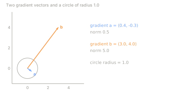
| Gradient clipping | "Capping the gradient norm" | Scaling down the gradient vector when its norm exceeds a threshold; prevents exploding gradient updates |
Further Reading
- Kingma & Ba, "Adam: A Method for Stochastic Optimization" (2014) — the original Adam paper with convergence analysis and the bias correction derivation
- Loshchilov & Hutter, "Decoupled Weight Decay Regularization" (2017) — proved that L2 regularization and weight decay are not equivalent in Adam, and proposed AdamW
- Smith, "Cyclical Learning Rates for Training Neural Networks" (2017) — introduced the LR range test and cyclical schedules that remove the need to tune a fixed learning rate
- Ruder, "An Overview of Gradient Descent Optimization Algorithms" (2016) — the best single survey of all optimizer variants, with clear comparisons and intuitions
Code
- main.py (python, 294 lines)