Regularization
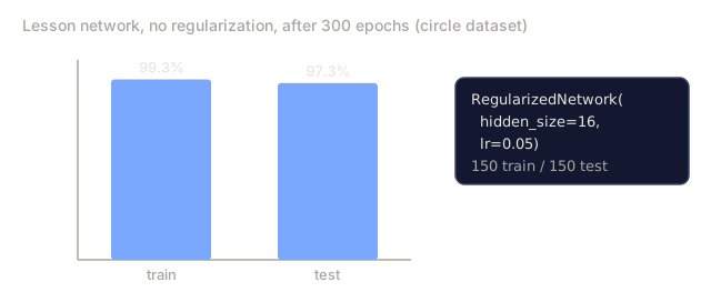
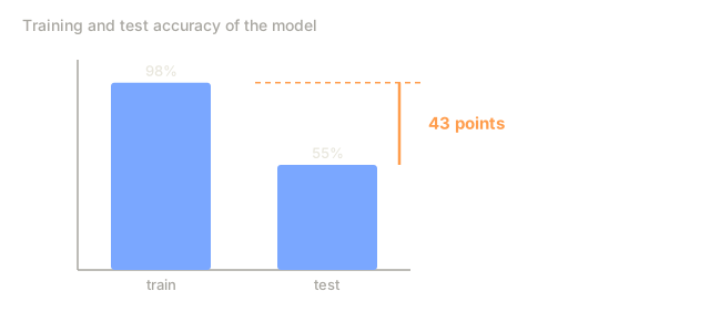
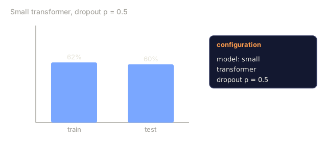
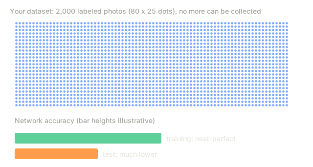
Your model hits 99% on training data and 60% on test data. That's not learning, that's memorization. Regularization is the tax you pay on complexity to force the model to generalize instead.
Learning Objectives
- Implement dropout with inverted scaling, L2 weight decay, batch normalization, layer normalization, and RMSNorm from scratch
- Measure the train-test accuracy gap and diagnose overfitting using regularization experiments
- Explain why transformers use LayerNorm instead of BatchNorm and why modern LLMs prefer RMSNorm
- Apply the correct combination of regularization techniques based on the severity of overfitting
The Problem
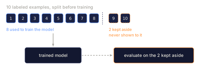
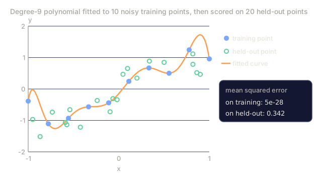
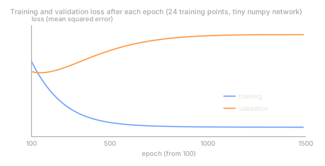
Overfitting is what happens when a model's training performance pulls way ahead of its test performance: the gap between the two is the tell that it memorized the training set's noise instead of learning patterns that generalize.
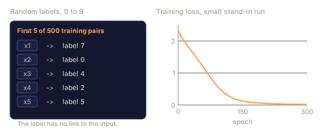
A neural network with enough parameters can memorize any dataset, and that's not a hypothetical. Zhang et al. (2017) trained standard networks on ImageNet with random labels and watched training loss drop to near zero. The networks memorized a million random input-output pairs with no real pattern behind them. Training loss was perfect. Test accuracy was zero.
The problem only gets worse as models scale up. GPT-3 has 175 billion parameters and trains on roughly 500 billion tokens. With that much capacity, the model can memorize large chunks of the training data verbatim. Without regularization, it would regurgitate training examples instead of learning patterns that generalize.
Every technique in this lesson closes that gap from a different angle. Dropout stops the network from leaning on any single neuron. Weight decay stops any single weight from growing too large. Batch normalization smooths the loss landscape so the optimizer lands on flatter, more generalizable minima. Layer normalization does the same job where batch normalization breaks down: small batches, variable-length sequences. RMSNorm gets there 10% faster by dropping the mean calculation entirely. Each technique on its own is simple. Put together, they're the difference between a model that memorizes and one that generalizes.

The Concept
The Overfitting Spectrum
Every model sits somewhere on a spectrum: underfitting (too simple to capture the pattern) on one end, overfitting (so complex it memorizes noise) on the other. The sweet spot sits between them, and regularization pushes a model toward it from the overfit side.

Dropout
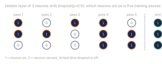
During training, randomly zero out each neuron's output with probability p. It's the simplest regularization technique in this lesson, and arguably the one with the most elegant interpretation.
output = activation(z) * mask where mask[i] ~ Bernoulli(1 - p)
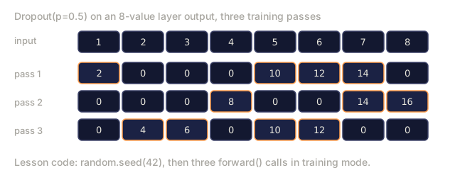
Bernoulli(1 - p) is just a weighted coin flip: it lands 1 with probability 1 - p and 0 otherwise, independently for every neuron on every forward pass. With p = 0.5, half the neurons get zeroed on every forward pass. The network can't predict which neurons will survive, so it's forced to learn redundant representations. That kills co-adaptation: neurons learning to depend on specific other neurons being present.
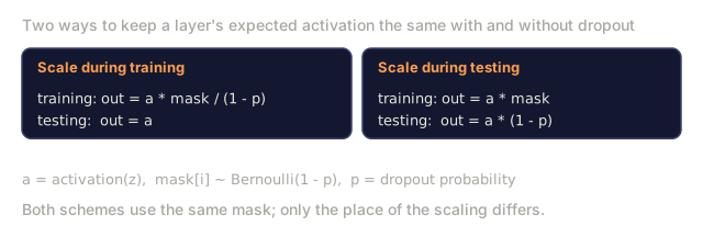
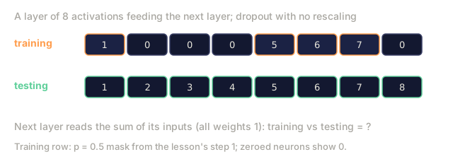
The ensemble interpretation is the deeper reason this works. A network with N neurons and dropout creates 2^N possible subnetworks, one for every combination of which neurons are on or off. Training with dropout approximately trains all 2^N of them at once, each on a different mini-batch. At test time you use every neuron (no dropout) and scale outputs by (1 - p) to match the expected value seen during training. That's the same as averaging the predictions of that entire 2^N-subnetwork ensemble, pulled out of a single trained model.
In practice, the scaling happens during training instead of testing. This is called inverted dropout:
During training:  output = activation(z) * mask / (1 - p)
During testing:   output = activation(z)   (no change needed)
It's cleaner this way: test code doesn't need to know dropout exists at all.
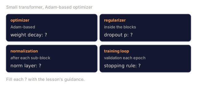
Default rates: p = 0.1 for transformers, p = 0.5 for MLPs, p = 0.2-0.3 for CNNs. Higher dropout means stronger regularization, and more risk of underfitting.
Weight Decay (L2 Regularization)
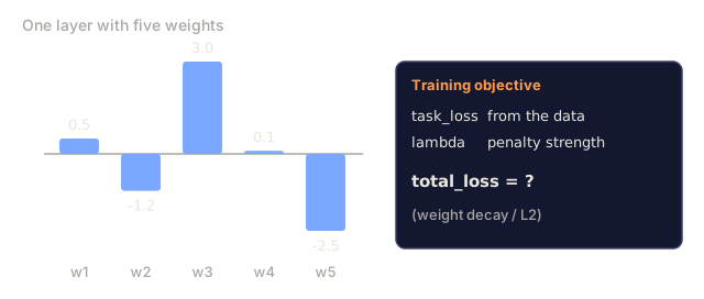
Add the squared magnitude of every weight to the loss:
total_loss = task_loss + (lambda / 2) * sum(w_i^2)
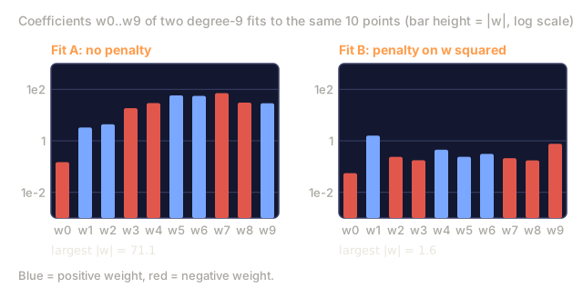
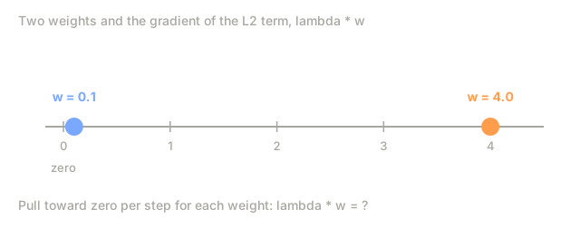
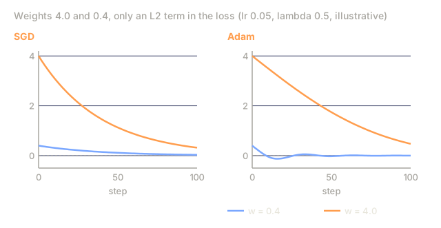
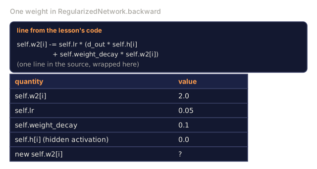
The gradient of that regularization term is lambda * w, so at every step each weight shrinks toward zero by an amount proportional to its own size. Large weights get penalized harder. The model gets pushed toward solutions where no single weight dominates.
Why does that help generalization? Overfit models tend to carry large weights that amplify noise in the training data. Weight decay keeps weights small, which caps the model's effective capacity and forces it to lean on stable, generalizable features instead of memorized quirks.
The lambda hyperparameter controls how hard that penalty bites. Typical values:
- 0.01 for AdamW on transformers
- 1e-4 for SGD on CNNs
- 0.1 for heavily overfit models
Lesson 06 covers this: weight decay and L2 regularization are equivalent under SGD, not under Adam. Always use AdamW (decoupled weight decay) whenever your optimizer is Adam-based.
Batch Normalization
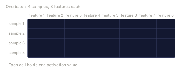
Normalize the output of each layer across the mini-batch, then hand it to the next layer.
For a mini-batch of activations at some layer:
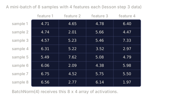
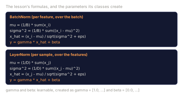
mu = (1/B) * sum(x_i)           (batch mean)
sigma^2 = (1/B) * sum((x_i - mu)^2)   (batch variance)
x_hat = (x_i - mu) / sqrt(sigma^2 + eps)   (normalize)
y = gamma * x_hat + beta        (scale and shift)
Gamma and beta are learnable parameters that let the network undo the normalization if that turns out to be the better move. Without them, you'd be forcing every layer's output to zero-mean, unit-variance, whether or not the network actually wants that.
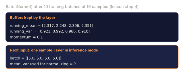
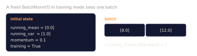
Training vs inference split: during training, mu and sigma come straight from the current mini-batch. During inference, you use running averages accumulated over training: an exponential moving average with momentum 0.1, so each update is 90% old value, 10% new.
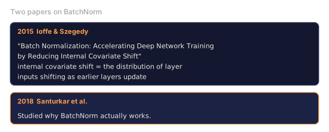
Why BatchNorm actually works is still debated. The original paper claimed it reduces "internal covariate shift," the distribution of layer inputs shifting as earlier layers update. Santurkar et al. (2018) showed that explanation is wrong. The real reason is that BatchNorm smooths the loss landscape: gradients get more predictive, the Lipschitz constants shrink (a bound on how sharply the loss can change from a small step, now tighter), and the optimizer can safely take bigger steps. That's why BatchNorm lets you push the learning rate higher and converge faster.
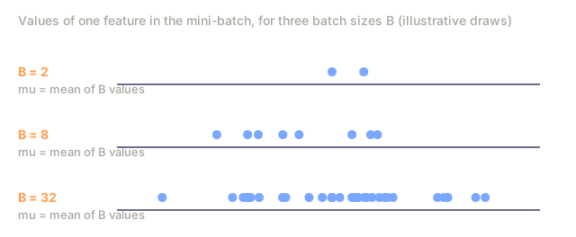
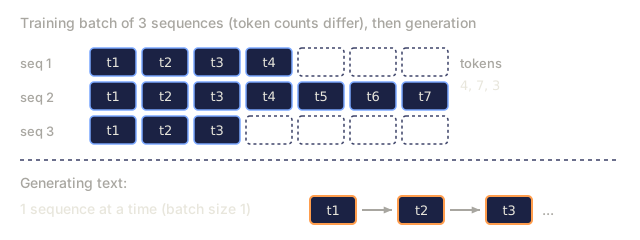
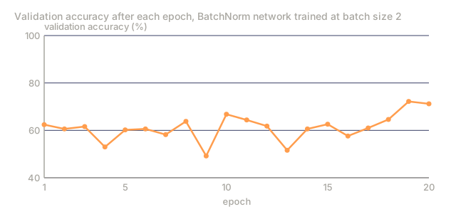
It also has a real limitation: it depends on batch statistics. At batch size 1, mean and variance are meaningless. Below 32, the statistics get noisy enough to hurt performance, which is a problem for tasks like object detection, where memory caps batch size, and language modeling, where sequence lengths vary.
Layer Normalization
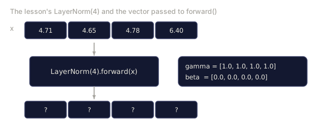
Normalize across features instead of across the batch. For a single sample:
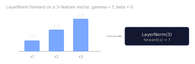
mu = (1/D) * sum(x_j)           (feature mean)
sigma^2 = (1/D) * sum((x_j - mu)^2)   (feature variance)
x_hat = (x_j - mu) / sqrt(sigma^2 + eps)
y = gamma * x_hat + beta
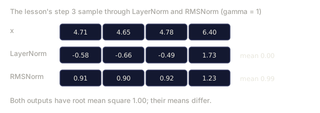
D is the feature dimension, and each sample gets normalized independently, with no dependence on batch size at all. That's exactly why transformers use LayerNorm instead of BatchNorm: sequences have variable lengths, batch size is often small (or exactly 1 during generation), and the computation stays identical between training and inference.
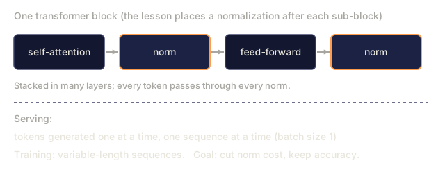
Transformers apply LayerNorm after each self-attention block and each feed-forward block (Post-LN), or before them (Pre-LN, which trains more stably).
RMSNorm
LayerNorm without the mean subtraction, proposed by Zhang & Sennrich (2019).
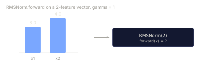
rms = sqrt((1/D) * sum(x_j^2))
y = gamma * x / rms
That's it. No mean computation, no beta parameter. The insight: re-centering, the mean subtraction inside LayerNorm, barely moves accuracy but costs real computation. Drop it and you get the same accuracy for about 10% less overhead.
LLaMA, LLaMA 2, LLaMA 3, Mistral, and most modern LLMs use RMSNorm instead of LayerNorm. At the scale of billions of parameters and trillions of tokens, that 10% adds up fast.
Normalization Comparison

Data Augmentation as Regularization
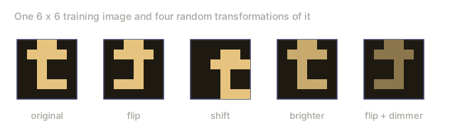
A change to the data, not the model: transform training inputs while keeping their labels fixed.
- Images: random crop, flip, rotation, color jitter, cutout
- Text: synonym replacement, back-translation, random deletion
- Audio: time stretch, pitch shift, noise addition
The effect works out the same as any other regularizer here. It inflates the effective size of the training set, so the model has a harder time memorizing specific examples. A model that only ever sees one version of an image can memorize it outright. A model that sees 50 augmented versions of that same image has no choice but to learn the structure that stays invariant across all of them.
Early Stopping
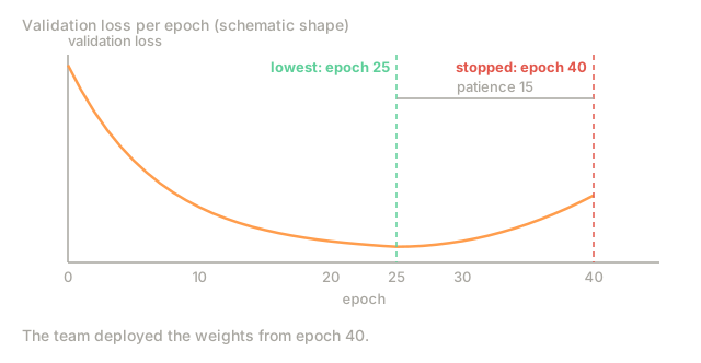
The simplest regularizer of all: stop training the moment validation loss starts climbing, since the model hasn't overfit yet at that exact point. In practice you track validation loss every epoch, save the best model, and keep training through a "patience" window (typically 5-20 epochs). If validation loss hasn't improved by the end of that window, you stop and reload the best saved model.
When to Apply What

Build It
Step 1: Dropout (Train and Eval Mode)
import random
import math


class Dropout:
    def __init__(self, p=0.5):
        self.p = p
        self.training = True
        self.mask = None

    def forward(self, x):
        if not self.training:
            return list(x)
        self.mask = []
        output = []
        for val in x:
            if random.random() < self.p:
                self.mask.append(0)
                output.append(0.0)
            else:
                self.mask.append(1)
                output.append(val / (1 - self.p))
        return output

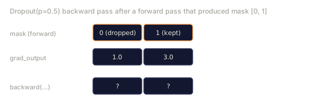
    def backward(self, grad_output):
        grads = []
        for g, m in zip(grad_output, self.mask):
            if m == 0:
                grads.append(0.0)
            else:
                grads.append(g / (1 - self.p))
        return grads
Step 2: L2 Weight Decay
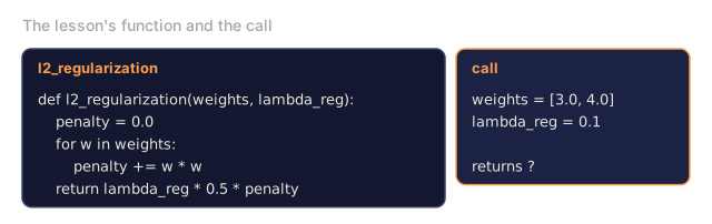
def l2_regularization(weights, lambda_reg):
    penalty = 0.0
    for w in weights:
        penalty += w * w
    return lambda_reg * 0.5 * penalty

def l2_gradient(weights, lambda_reg):
    return [lambda_reg * w for w in weights]
Step 3: Batch Normalization
class BatchNorm:
    def __init__(self, num_features, momentum=0.1, eps=1e-5):
        self.gamma = [1.0] * num_features
        self.beta = [0.0] * num_features
        self.eps = eps
        self.momentum = momentum
        self.running_mean = [0.0] * num_features
        self.running_var = [1.0] * num_features
        self.training = True
        self.num_features = num_features

    def forward(self, batch):
        batch_size = len(batch)
        if self.training:
            mean = [0.0] * self.num_features
            for sample in batch:
                for j in range(self.num_features):
                    mean[j] += sample[j]
            mean = [m / batch_size for m in mean]

            var = [0.0] * self.num_features
            for sample in batch:
                for j in range(self.num_features):
                    var[j] += (sample[j] - mean[j]) ** 2
            var = [v / batch_size for v in var]

            for j in range(self.num_features):
                self.running_mean[j] = (1 - self.momentum) * self.running_mean[j] + self.momentum * mean[j]
                self.running_var[j] = (1 - self.momentum) * self.running_var[j] + self.momentum * var[j]
        else:
            mean = list(self.running_mean)
            var = list(self.running_var)

        self.x_hat = []
        output = []
        for sample in batch:
            normalized = []
            out_sample = []
            for j in range(self.num_features):
                x_h = (sample[j] - mean[j]) / math.sqrt(var[j] + self.eps)
                normalized.append(x_h)
                out_sample.append(self.gamma[j] * x_h + self.beta[j])
            self.x_hat.append(normalized)
            output.append(out_sample)
        return output
Step 4: Layer Normalization
class LayerNorm:
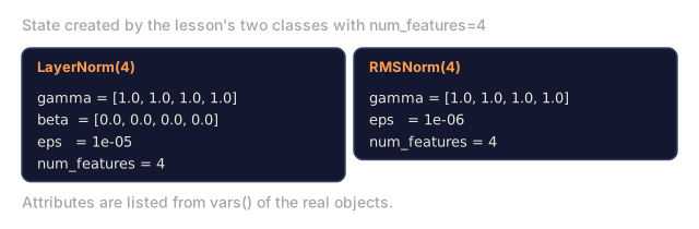
    def __init__(self, num_features, eps=1e-5):
        self.gamma = [1.0] * num_features
        self.beta = [0.0] * num_features
        self.eps = eps
        self.num_features = num_features

    def forward(self, x):
        mean = sum(x) / len(x)
        var = sum((xi - mean) ** 2 for xi in x) / len(x)

        self.x_hat = []
        output = []
        for j in range(self.num_features):
            x_h = (x[j] - mean) / math.sqrt(var + self.eps)
            self.x_hat.append(x_h)
            output.append(self.gamma[j] * x_h + self.beta[j])
        return output
Step 5: RMSNorm
class RMSNorm:
    def __init__(self, num_features, eps=1e-6):
        self.gamma = [1.0] * num_features
        self.eps = eps
        self.num_features = num_features

    def forward(self, x):
        rms = math.sqrt(sum(xi * xi for xi in x) / len(x) + self.eps)
        output = []
        for j in range(self.num_features):
            output.append(self.gamma[j] * x[j] / rms)
        return output
Step 6: Training With and Without Regularization
def sigmoid(x):
    x = max(-500, min(500, x))
    return 1.0 / (1.0 + math.exp(-x))


def make_circle_data(n=200, seed=42):
    random.seed(seed)
    data = []
    for _ in range(n):
        x = random.uniform(-2, 2)
        y = random.uniform(-2, 2)
        label = 1.0 if x * x + y * y < 1.5 else 0.0
        data.append(([x, y], label))
    return data


class RegularizedNetwork:
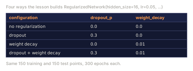
    def __init__(self, hidden_size=16, lr=0.05, dropout_p=0.0, weight_decay=0.0):
        random.seed(0)
        self.hidden_size = hidden_size
        self.lr = lr
        self.dropout_p = dropout_p
        self.weight_decay = weight_decay
        self.dropout = Dropout(p=dropout_p) if dropout_p > 0 else None

        self.w1 = [[random.gauss(0, 0.5) for _ in range(2)] for _ in range(hidden_size)]
        self.b1 = [0.0] * hidden_size
        self.w2 = [random.gauss(0, 0.5) for _ in range(hidden_size)]
        self.b2 = 0.0

    def forward(self, x, training=True):
        self.x = x
        self.z1 = []
        self.h = []
        for i in range(self.hidden_size):
            z = self.w1[i][0] * x[0] + self.w1[i][1] * x[1] + self.b1[i]
            self.z1.append(z)
            self.h.append(max(0.0, z))

        if self.dropout and training:
            self.dropout.training = True
            self.h = self.dropout.forward(self.h)
        elif self.dropout:
            self.dropout.training = False
            self.h = self.dropout.forward(self.h)

        self.z2 = sum(self.w2[i] * self.h[i] for i in range(self.hidden_size)) + self.b2
        self.out = sigmoid(self.z2)
        return self.out

    def backward(self, target):
        eps = 1e-15
        p = max(eps, min(1 - eps, self.out))
        d_loss = -(target / p) + (1 - target) / (1 - p)
        d_sigmoid = self.out * (1 - self.out)
        d_out = d_loss * d_sigmoid

        for i in range(self.hidden_size):
            d_relu = 1.0 if self.z1[i] > 0 else 0.0
            d_h = d_out * self.w2[i] * d_relu
            self.w2[i] -= self.lr * (d_out * self.h[i] + self.weight_decay * self.w2[i])
            for j in range(2):
                self.w1[i][j] -= self.lr * (d_h * self.x[j] + self.weight_decay * self.w1[i][j])
            self.b1[i] -= self.lr * d_h
        self.b2 -= self.lr * d_out

    def evaluate(self, data):
        correct = 0
        total_loss = 0.0
        for x, y in data:
            pred = self.forward(x, training=False)
            eps = 1e-15
            p = max(eps, min(1 - eps, pred))
            total_loss += -(y * math.log(p) + (1 - y) * math.log(1 - p))
            if (pred >= 0.5) == (y >= 0.5):
                correct += 1
        return total_loss / len(data), correct / len(data) * 100

    def train_model(self, train_data, test_data, epochs=300):
        history = []
        for epoch in range(epochs):
            total_loss = 0.0
            correct = 0
            for x, y in train_data:
                pred = self.forward(x, training=True)
                self.backward(y)
                eps = 1e-15
                p = max(eps, min(1 - eps, pred))
                total_loss += -(y * math.log(p) + (1 - y) * math.log(1 - p))
                if (pred >= 0.5) == (y >= 0.5):
                    correct += 1
            train_loss = total_loss / len(train_data)
            train_acc = correct / len(train_data) * 100
            test_loss, test_acc = self.evaluate(test_data)
            history.append((train_loss, train_acc, test_loss, test_acc))
            if epoch % 75 == 0 or epoch == epochs - 1:
                gap = train_acc - test_acc
                print(f"    Epoch {epoch:3d}: train_acc={train_acc:.1f}%, test_acc={test_acc:.1f}%, gap={gap:.1f}%")
        return history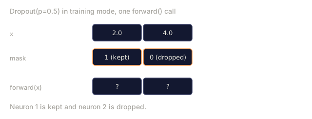
Use It
PyTorch ships all of this as modules:
import torch
import torch.nn as nn

model = nn.Sequential(
    nn.Linear(784, 256),
    nn.BatchNorm1d(256),
    nn.ReLU(),
    nn.Dropout(0.3),
    nn.Linear(256, 128),
    nn.BatchNorm1d(128),
    nn.ReLU(),
    nn.Dropout(0.3),
    nn.Linear(128, 10),
)

model.train()
out_train = model(torch.randn(32, 784))

model.eval()
out_test = model(torch.randn(1, 784))
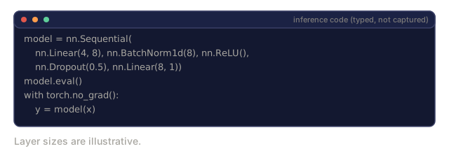
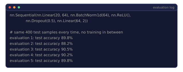
The model.train() / model.eval() toggle matters more than it looks. It switches dropout on or off and tells BatchNorm whether to trust batch statistics or running statistics. Forgetting model.eval() before inference is one of the most common bugs in deep learning: your test accuracy fluctuates randomly because dropout is still firing and BatchNorm is still reading mini-batch statistics instead of the stable running averages.
Transformers follow a different pattern:
class TransformerBlock(nn.Module):
    def __init__(self, d_model=512, nhead=8, dropout=0.1):
        super().__init__()
        self.attention = nn.MultiheadAttention(d_model, nhead, dropout=dropout)
        self.norm1 = nn.LayerNorm(d_model)
        self.ff = nn.Sequential(
            nn.Linear(d_model, d_model * 4),
            nn.GELU(),
            nn.Linear(d_model * 4, d_model),
            nn.Dropout(dropout),
        )
        self.norm2 = nn.LayerNorm(d_model)
        self.dropout = nn.Dropout(dropout)

    def forward(self, x):
        attended, _ = self.attention(x, x, x)
        x = self.norm1(x + self.dropout(attended))
        x = self.norm2(x + self.ff(x))
        return x
LayerNorm, not BatchNorm. Dropout p=0.1, not p=0.5. These are the transformer defaults.
Ship It
This lesson produces:
outputs/prompt-regularization-advisor.md: a prompt that diagnoses overfitting and recommends the right regularization strategy
Exercises
-
Implement spatial dropout for 2D data: instead of dropping individual neurons, drop entire feature channels. Simulate this by treating groups of consecutive features as channels and dropping whole groups. Compare the train-test gap to standard dropout on the circle dataset with hidden_size=32.
-
Implement label smoothing from lesson 05 combined with dropout from this lesson. Train with four configurations: neither, dropout only, label smoothing only, both. Measure the final train-test accuracy gap for each. Which combination gives the smallest gap?
-
Add a BatchNorm layer between the hidden layer and the activation in your circle-dataset network. Train with and without BatchNorm at learning rates 0.01, 0.05, and 0.1. BatchNorm should allow stable training at higher learning rates where the vanilla network diverges.
-
Implement early stopping: track test loss each epoch, save the best weights, and stop if test loss hasn't improved for 20 epochs. Run the regularized network for 1000 epochs. Report which epoch had the best test accuracy and how many epochs of computation you saved.
-
Compare LayerNorm vs RMSNorm on a 4-layer network (not just 2). Initialize both with the same weights. Train for 200 epochs and compare final accuracy, training speed (time per epoch), and gradient magnitudes at the first layer. Verify that RMSNorm is faster with the same accuracy.
Key Terms
| Term | What people say | What it actually means |
|---|---|---|
| Overfitting | "Model memorized the data" | When a model's training performance significantly exceeds its test performance, indicating it learned noise rather than signal |
| Regularization | "Preventing overfitting" | Any technique that constrains model complexity to improve generalization: dropout, weight decay, normalization, augmentation |
| Dropout | "Random neuron deletion" | Zeroing random neurons during training with probability p, forcing redundant representations; equivalent to training an ensemble |
| Weight decay | "L2 penalty" | Shrinking all weights toward zero by subtracting lambda * w at each step; penalizes complexity through weight magnitude |
| Batch normalization | "Normalize per batch" | Normalizing layer outputs across the batch dimension using batch statistics during training and running averages during inference |
| Layer normalization | "Normalize per sample" | Normalizing across features within each sample; batch-independent, used in transformers where batch size varies |
| RMSNorm | "LayerNorm without the mean" | Root mean square normalization; drops the mean subtraction from LayerNorm for 10% speedup with equal accuracy |
| Early stopping | "Stop before overfit" | Halting training when validation loss stops improving; the simplest regularizer, often used alongside others |
| Data augmentation | "More data from less" | Transforming training inputs (flip, crop, noise) to increase effective dataset size and force invariance learning |
| Generalization gap | "Train-test split" | The difference between training and test performance; regularization aims to minimize this gap |
Further Reading
- Srivastava et al., "Dropout: A Simple Way to Prevent Neural Networks from Overfitting" (2014) — the original dropout paper, with the ensemble interpretation and extensive experiments
- Ioffe & Szegedy, "Batch Normalization: Accelerating Deep Network Training by Reducing Internal Covariate Shift" (2015) — introduced BatchNorm and its training procedure, one of the most cited deep learning papers
- Zhang & Sennrich, "Root Mean Square Layer Normalization" (2019) — showed RMSNorm matches LayerNorm accuracy with reduced computation, adopted by LLaMA and Mistral
- Zhang et al., "Understanding Deep Learning Requires Rethinking Generalization" (2017) — the landmark paper showing neural networks can memorize random labels, challenging traditional views of generalization
Code
- main.py (python, 348 lines)