Weight Initialization and Training Stability
Initialize wrong and training never starts. Initialize right and 50 layers train as smoothly as 3.
Learning Objectives
- Implement zero, random, Xavier/Glorot, and Kaiming/He initialization strategies and measure their effect on activation magnitudes through 50 layers
- Derive why Xavier init uses Var(w) = 2/(fan_in + fan_out) and Kaiming uses Var(w) = 2/fan_in
- Demonstrate the symmetry problem with zero initialization and explain why random scale alone is insufficient
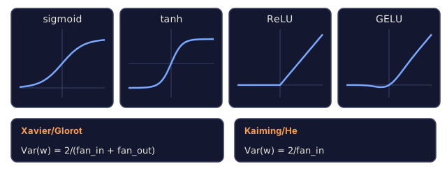
- Match the correct initialization strategy to the activation function: Xavier for sigmoid/tanh, Kaiming for ReLU/GELU
The Problem
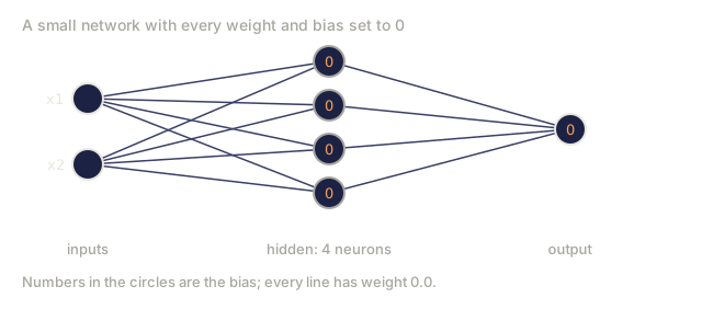
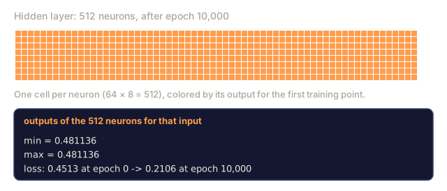
Initialize all weights to zero. Nothing learns. Every neuron computes the same function, receives the same gradient, and updates identically. After 10,000 epochs, your 512-neuron hidden layer is still 512 copies of the same neuron. You paid for 512 parameters and got 1.
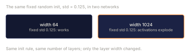
Initialize them too large. Activations explode through the network. By layer 10, values hit 1e15. By layer 20, they overflow to infinity. Gradients follow the same trajectory in reverse.
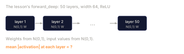
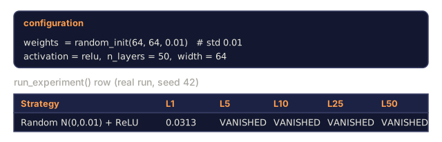
Initialize them randomly from a standard normal distribution. Works for 3 layers. At 50 layers, the signal collapses to zero or detonates to infinity depending on whether the random scale was slightly too small or slightly too large. The boundary between "works" and "broken" is razor-thin.
Weight initialization is the most underrated decision in deep learning. Architecture gets papers. Optimizers get blog posts. Initialization gets a footnote. But get it wrong and nothing else matters: your network is dead before training begins.
The Concept
The Symmetry Problem
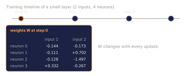
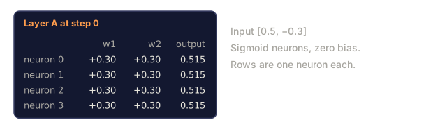
Symmetry is what happens when every neuron in a layer starts out identical and therefore stays identical. Each neuron runs the same computation: multiply inputs by weights, add a bias, apply an activation. If every weight starts at the same value (zero is the extreme case), every neuron produces the same output, receives the same gradient during backpropagation, and changes by the same amount at every update step. Hundreds of parameters, moving in lockstep, forever.
Random initialization is the brute-force fix: give each neuron a different starting point in weight space so each one settles on a different feature.
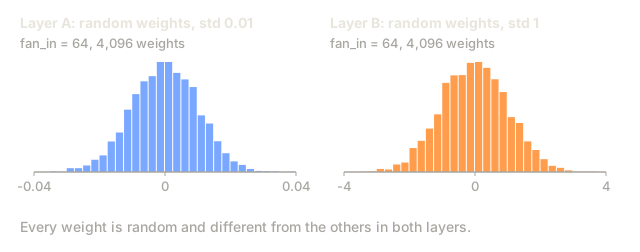
But "random" alone isn't enough. The scale of that randomness decides whether the network trains at all.
Variance Propagation Through Layers
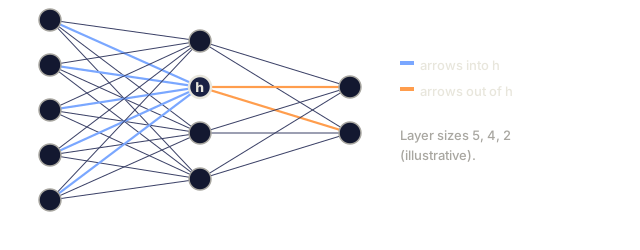
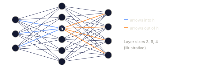
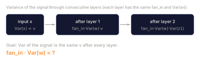
Consider a single layer with fan_in inputs:
z = w1*x1 + w2*x2 + ... + w_n*x_n
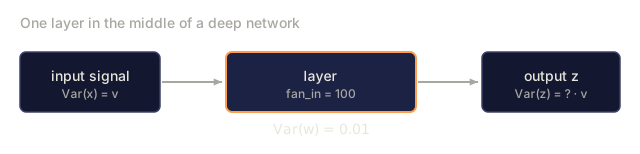
If each weight wi is drawn from a distribution with variance Var(w) and each input xi has variance Var(x), the output variance is:
Var(z) = fan_in * Var(w) * Var(x)
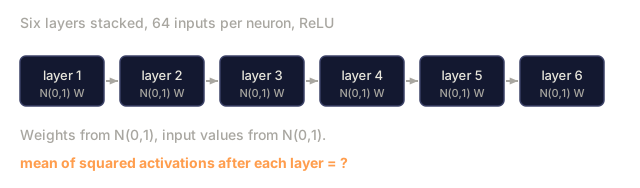
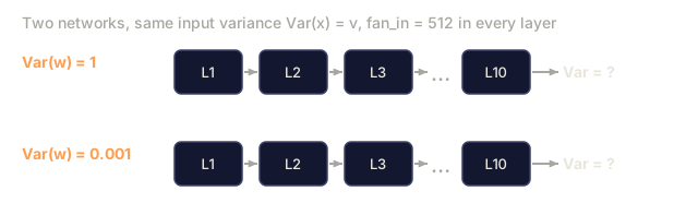
If Var(w) = 1 and fan_in = 512, the output variance is 512x the input variance. After 10 layers: 512^10 = 1.2e27. Your signal has exploded.
If Var(w) = 0.001, the output variance shrinks by 0.001 * 512 = 0.512 per layer. After 10 layers: 0.512^10 = 0.00124. Your signal has vanished.
The goal: choose Var(w) so that Var(z) = Var(x). Signal magnitude stays constant across layers.
Xavier/Glorot Initialization
Glorot and Bengio (2010) derived the solution for sigmoid and tanh activations. To keep variance constant in both the forward and backward pass:
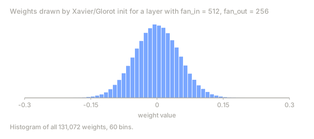
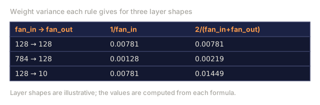
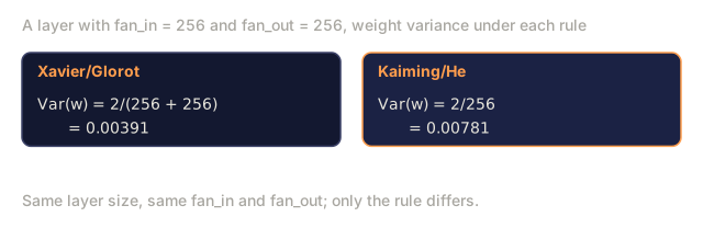
Var(w) = 2 / (fan_in + fan_out)
In practice, weights are drawn from:
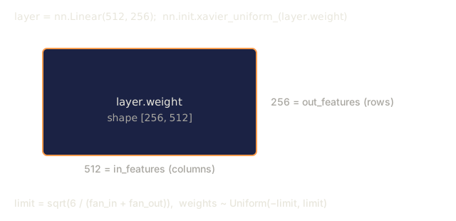
w ~ Uniform(-limit, limit) where limit = sqrt(6 / (fan_in + fan_out))
or:
w ~ Normal(0, sqrt(2 / (fan_in + fan_out)))
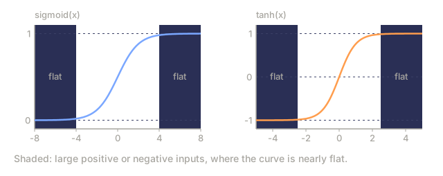
This works because sigmoid and tanh are roughly linear near zero, where properly initialized activations live. The variance stays stable through dozens of layers.
Kaiming/He Initialization
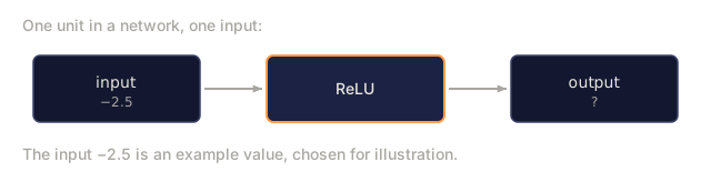
ReLU kills half the outputs (everything negative becomes zero). The effective fan_in is halved because on average half the inputs are zeroed. Xavier init doesn't account for this: it underestimates the variance needed.
He et al. (2015) adjusted the formula:
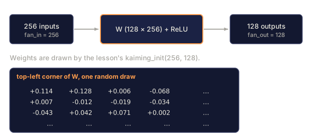
Var(w) = 2 / fan_in
Weights are drawn from:
w ~ Normal(0, sqrt(2 / fan_in))
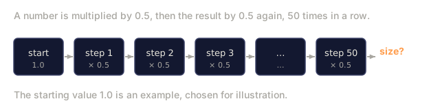
The factor of 2 compensates for ReLU zeroing half the activations. Without it, the signal shrinks by ~0.5x per layer. With 50 layers: 0.5^50 = 8.8e-16. Kaiming init prevents this.
Transformer Initialization
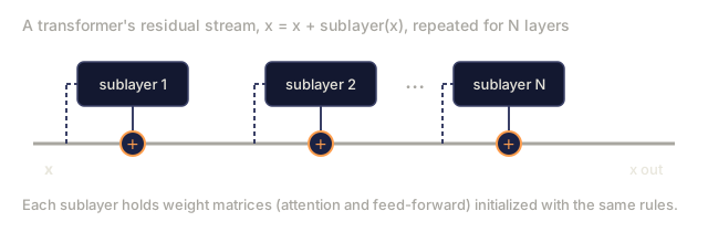
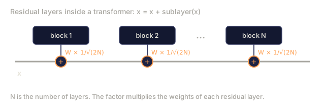
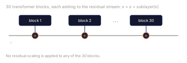
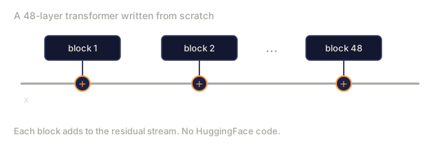
GPT-2 introduced a different pattern. Residual connections add the output of each sub-layer to its input:
x = x + sublayer(x)
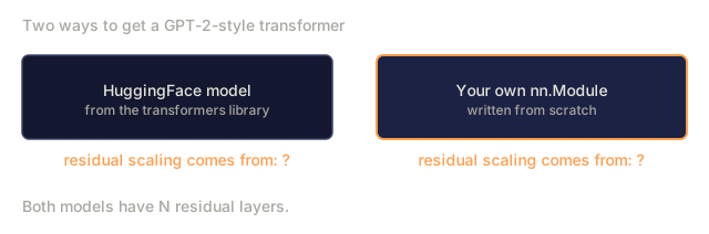
Each addition increases variance. With N residual layers, variance grows proportionally to N. GPT-2 scales the weights of residual layers by 1/sqrt(2N), where N is the number of layers. This keeps the accumulated signal magnitude stable.
Llama 3 (405B parameters, 126 layers) uses a similar scheme. Without this scaling, the residual stream would grow unbounded through 126 layers of attention and feedforward blocks.

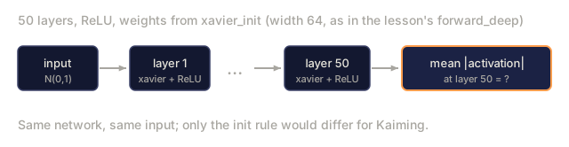
Activation Magnitude Through 50 Layers

Choosing the Right Init

Build It
Step 1: Initialization Strategies
Four ways to initialize a weight matrix. Each returns a list of lists (a 2D matrix) with fan_in columns and fan_out rows.
import math
import random


def zero_init(fan_in, fan_out):
    return [[0.0 for _ in range(fan_in)] for _ in range(fan_out)]


def random_init(fan_in, fan_out, scale=1.0):
    return [[random.gauss(0, scale) for _ in range(fan_in)] for _ in range(fan_out)]


def xavier_init(fan_in, fan_out):
    std = math.sqrt(2.0 / (fan_in + fan_out))
    return [[random.gauss(0, std) for _ in range(fan_in)] for _ in range(fan_out)]


def kaiming_init(fan_in, fan_out):
    std = math.sqrt(2.0 / fan_in)
    return [[random.gauss(0, std) for _ in range(fan_in)] for _ in range(fan_out)]
Step 2: Activation Functions
We need sigmoid, tanh, and ReLU to test each init strategy with its intended activation.
def sigmoid(x):
    x = max(-500, min(500, x))
    return 1.0 / (1.0 + math.exp(-x))


def tanh_act(x):
    return math.tanh(x)


def relu(x):
    return max(0.0, x)
Step 3: Forward Pass Through 50 Layers
Pass random data through a deep network and measure mean activation magnitude at each layer.
def forward_deep(init_fn, activation_fn, n_layers=50, width=64, n_samples=100):
    random.seed(42)
    layer_magnitudes = []

    inputs = [[random.gauss(0, 1) for _ in range(width)] for _ in range(n_samples)]

    for layer_idx in range(n_layers):
        weights = init_fn(width, width)
        biases = [0.0] * width

        new_inputs = []
        for sample in inputs:
            output = []
            for neuron_idx in range(width):
                z = sum(weights[neuron_idx][j] * sample[j] for j in range(width)) + biases[neuron_idx]
                output.append(activation_fn(z))
            new_inputs.append(output)
        inputs = new_inputs

        magnitudes = []
        for sample in inputs:
            magnitudes.append(sum(abs(v) for v in sample) / width)
        mean_mag = sum(magnitudes) / len(magnitudes)
        layer_magnitudes.append(mean_mag)

    return layer_magnitudes
Step 4: The Experiment
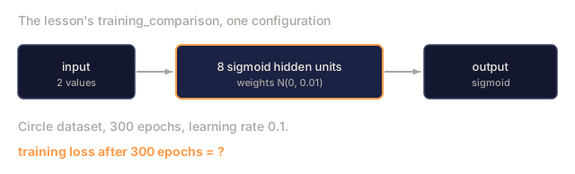
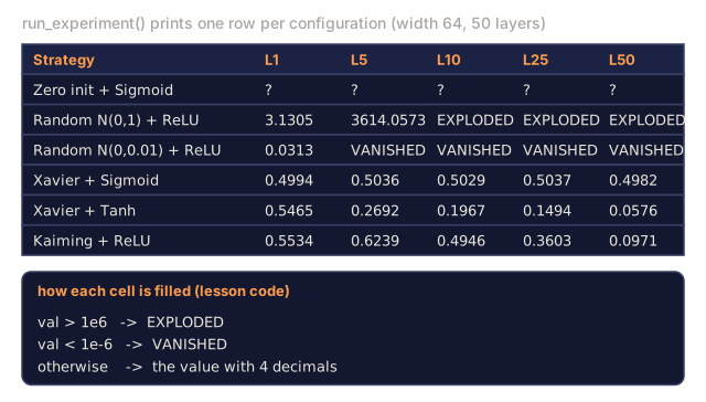
Run all combinations: zero init, random N(0,1), random N(0,0.01), Xavier with sigmoid, Xavier with tanh, Kaiming with ReLU. Print the magnitude at key layers.
def run_experiment():
    configs = [
        ("Zero init + Sigmoid", lambda fi, fo: zero_init(fi, fo), sigmoid),
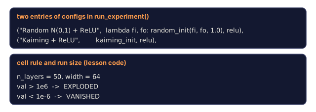
        ("Random N(0,1) + ReLU", lambda fi, fo: random_init(fi, fo, 1.0), relu),
        ("Random N(0,0.01) + ReLU", lambda fi, fo: random_init(fi, fo, 0.01), relu),
        ("Xavier + Sigmoid", xavier_init, sigmoid),
        ("Xavier + Tanh", xavier_init, tanh_act),
        ("Kaiming + ReLU", kaiming_init, relu),
    ]

    print(f"{'Strategy':<30} {'L1':>10} {'L5':>10} {'L10':>10} {'L25':>10} {'L50':>10}")
    print("-" * 80)

    for name, init_fn, act_fn in configs:
        mags = forward_deep(init_fn, act_fn)
        row = f"{name:<30}"
        for idx in [0, 4, 9, 24, 49]:
            val = mags[idx]
            if val > 1e6:
                row += f" {'EXPLODED':>10}"
            elif val < 1e-6:
                row += f" {'VANISHED':>10}"
            else:
                row += f" {val:>10.4f}"
        print(row)
Step 5: Symmetry Demonstration
Show that zero init produces identical neurons.
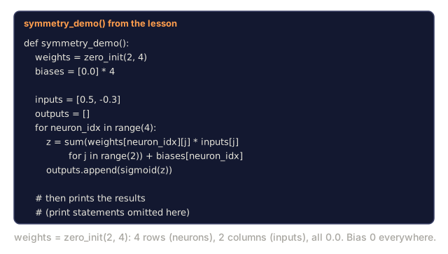
def symmetry_demo():
    random.seed(42)
    weights = zero_init(2, 4)
    biases = [0.0] * 4

    inputs = [0.5, -0.3]
    outputs = []
    for neuron_idx in range(4):
        z = sum(weights[neuron_idx][j] * inputs[j] for j in range(2)) + biases[neuron_idx]
        outputs.append(sigmoid(z))

    print("\nSymmetry Demo (4 neurons, zero init):")
    for i, out in enumerate(outputs):
        print(f"  Neuron {i}: output = {out:.6f}")
    all_same = all(abs(outputs[i] - outputs[0]) < 1e-10 for i in range(len(outputs)))
    print(f"  All identical: {all_same}")
    print(f"  Effective parameters: 1 (not {len(weights) * len(weights[0])})")
Step 6: Layer-by-Layer Magnitude Report
Print a visual bar chart of activation magnitudes through 50 layers.
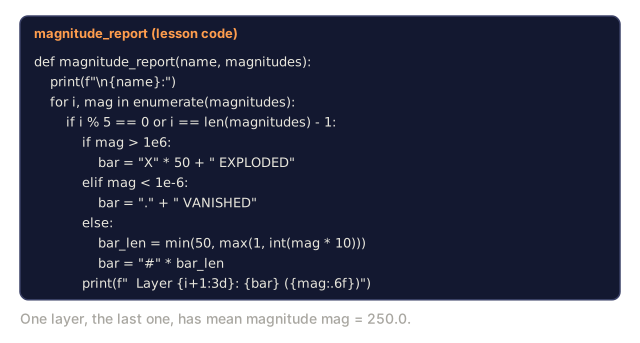
def magnitude_report(name, magnitudes):
    print(f"\n{name}:")
    for i, mag in enumerate(magnitudes):
        if i % 5 == 0 or i == len(magnitudes) - 1:
            if mag > 1e6:
                bar = "X" * 50 + " EXPLODED"
            elif mag < 1e-6:
                bar = "." + " VANISHED"
            else:
                bar_len = min(50, max(1, int(mag * 10)))
                bar = "#" * bar_len
            print(f"  Layer {i+1:3d}: {bar} ({mag:.6f})")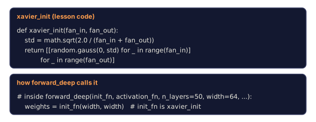
Use It
PyTorch provides these as built-in functions:
import torch
import torch.nn as nn

layer = nn.Linear(512, 256)

nn.init.xavier_uniform_(layer.weight)
nn.init.xavier_normal_(layer.weight)

nn.init.kaiming_uniform_(layer.weight, nonlinearity='relu')
nn.init.kaiming_normal_(layer.weight, nonlinearity='relu')

nn.init.zeros_(layer.bias)
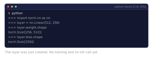
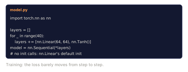
When you call nn.Linear(512, 256), PyTorch defaults to Kaiming uniform initialization. That's why most simple networks "just work": PyTorch already made the right choice. But when you build custom architectures or go deeper than 20 layers, you need to understand what's happening and potentially override the default.
For transformers, HuggingFace models typically handle initialization in their _init_weights method. GPT-2's implementation scales residual projections by 1/sqrt(N). If you're building a transformer from scratch, you need to add this yourself.
Ship It
This lesson produces:
outputs/prompt-init-strategy.md, a prompt that diagnoses weight initialization problems and recommends the right strategy
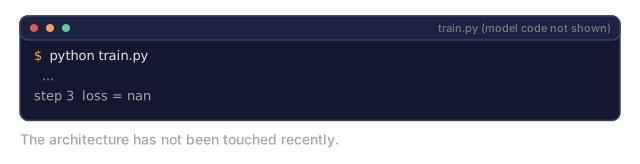
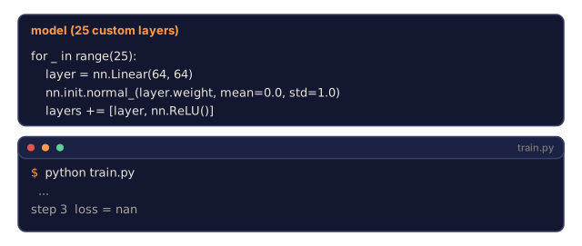
The bug this lesson is really about rarely announces itself as an initialization bug. It shows up as a loss that's NaN by step three, or a network that sits at exactly chance-level accuracy for a thousand epochs and never budges. Most people burn a day tuning the learning rate before they think to check what their weights started at. Check init first. It's a five-second look compared to a day of blind hyperparameter search.
The other trap is trusting PyTorch's defaults past the point where they still apply. nn.Linear ships with Kaiming uniform, which is why toy networks train fine on the first try and give you a false sense that init is a solved problem. That confidence runs out the moment you write a custom layer, stack more than about 20 of them, or add residual connections without scaling them, because those are exactly the cases the default's assumptions don't cover. That's when the variance math in this lesson stops being trivia and starts being the thing that decides whether your network trains at all.
Exercises
-
Add LeCun initialization (Var = 1/fan_in, designed for SELU activation). Run the 50-layer experiment with LeCun init + tanh and compare to Xavier + tanh.
-
Implement the GPT-2 residual scaling: multiply the output of each layer by 1/sqrt(2*N) before adding to the residual stream. Run 50 layers with and without scaling, measure how fast the residual magnitude grows.
-
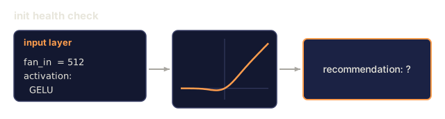
Create an "init health check" function that takes a network's layer dimensions and activation type, then recommends the correct initialization and warns if the current init will cause problems.
-
Run the experiment with fan_in = 16 vs fan_in = 1024. Xavier and Kaiming adapt to fan_in, but random init doesn't. Show how the gap between "works" and "breaks" widens with larger layers.
-
Implement orthogonal initialization (generate a random matrix, compute its SVD, use the orthogonal matrix U). Compare to Kaiming for ReLU networks at 50 layers.
Key Terms
| Term | What people say | What it actually means |
|---|---|---|
| Weight initialization | "Set starting weights randomly" | The strategy for choosing initial weight values that determines whether a network can train at all |
| Symmetry breaking | "Make neurons different" | Using random initialization to ensure neurons learn distinct features instead of computing identical functions |
| Fan-in | "Number of inputs to a neuron" | The number of incoming connections, which determines how input variance accumulates in the weighted sum |
| Fan-out | "Number of outputs from a neuron" | The number of outgoing connections, relevant for maintaining gradient variance during backpropagation |
| Xavier/Glorot init | "The sigmoid initialization" | Var(w) = 2/(fan_in + fan_out), designed to preserve variance through sigmoid and tanh activations |
| Kaiming/He init | "The ReLU initialization" | Var(w) = 2/fan_in, accounts for ReLU zeroing half the activations |
| Variance propagation | "How signals grow or shrink through layers" | The mathematical analysis of how activation variance changes layer by layer based on weight scale |
| Residual scaling | "GPT-2's init trick" | Scaling residual connection weights by 1/sqrt(2N) to prevent variance growth through N transformer layers |
| Dead network | "Nothing trains" | A network where poor initialization causes all gradients to be zero or all activations to saturate |
| Exploding activations | "Values go to infinity" | When weight variance is too high, causing activation magnitudes to grow exponentially through layers |
Further Reading
- Glorot & Bengio, "Understanding the difficulty of training deep feedforward neural networks" (2010) — the original Xavier initialization paper with variance analysis
- He et al., "Delving Deep into Rectifiers" (2015) — introduced Kaiming initialization for ReLU networks
- Radford et al., "Language Models are Unsupervised Multitask Learners" (2019) — GPT-2 paper with residual scaling initialization
- Mishkin & Matas, "All You Need is a Good Init" (2016) — layer-sequential unit-variance initialization, an empirical alternative to analytical formulas
Code
- main.py (python, 274 lines)