BuildPython

Build Your Own Mini Framework

You've built neurons, layers, networks, backprop, activations, loss functions, optimizers, regularization, initialization, and LR schedules, all as separate pieces. Now wire them together into a framework. Not PyTorch. Not TensorFlow. Yours.

TIME: ~120 minutesPREREQUISITES: All of Phase 03 (Lessons 01-09)

Learning Objectives

Build a complete deep learning framework (~650 lines) with Module, Linear, ReLU, Sigmoid, Dropout, BatchNorm, Sequential, loss functions, optimizers, and DataLoader
Explain the Module abstraction (forward, backward, parameters) and why train/eval mode toggling is necessary
Wire all components into a working training loop that trains a 4-layer network on circle classification
Map each component of your framework to its PyTorch equivalent (nn.Module, nn.Sequential, optim.Adam, DataLoader)

The Problem

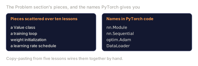
You have ten lessons of building blocks scattered across separate files. A Value class here, a training loop there, weight initialization in another file, learning rate schedules in yet another. To train a network, you copy-paste from five different lessons and wire them together by hand.

That's what frameworks solve. PyTorch gives you nn.Module, nn.Sequential, optim.Adam, DataLoader, and a training loop pattern that ties them together. TensorFlow gives you keras.Layer, keras.Sequential, keras.optimizers.Adam. These aren't magic. They're organizational patterns that let you define, train, and evaluate networks without reinventing the plumbing every time.

You're going to build the same thing in ~650 lines of Python. No numpy. No external dependencies. A framework that can define any feedforward network, train it with SGD or Adam, batch the data, apply dropout and batch normalization, use any activation, and schedule the learning rate.

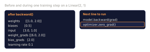
When you finish, you'll understand exactly what happens when you write model = nn.Sequential(...) in PyTorch: why model.train() and model.eval() exist, and why optimizer.zero_grad() is a separate call instead of something the framework does for you. You'll understand all of it, because you built all of it.

Warm-up0/3

1. A weight's gradient is positive, meaning that raising the weight would raise the loss. What does plain gradient descent do to that weight?Warm-up

A U-shaped loss curve against one weight, with the current weight marked on the right branch and a dashed tangent line rising to the right, labelled gradient = +3.0. — Illustrative curve and numbers.

2. When you train a neural network, what is one epoch?Warm-up

Twelve numbered training examples drawn in three groups of four with a weight update marked under each group, and three separate held-out test examples on the right. — Illustrative sizes.

3. A network must output one number between 0 and 1 that can be read as the probability of class 1. Which output activation fits?Warm-up

Illustrative scores.

Check: The Problem0/1

1. What role do frameworks like PyTorch and TensorFlow play for someone who already knows the pieces of a neural network?Explain

Two cards: on the left four pieces written in earlier lessons (a Value class, a training loop, weight initialization, a learning rate schedule), on the right four PyTorch names (nn.Module, nn.Sequential, optim.Adam, DataLoader). — Items taken from the lesson's Problem section.

The Concept

The Module Abstraction

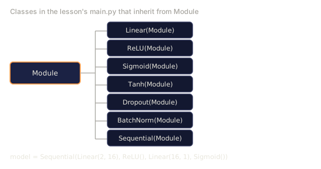
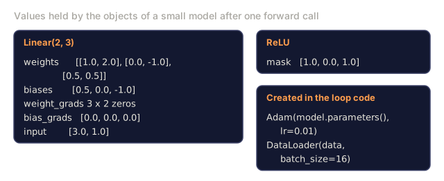
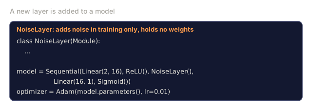
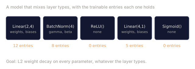
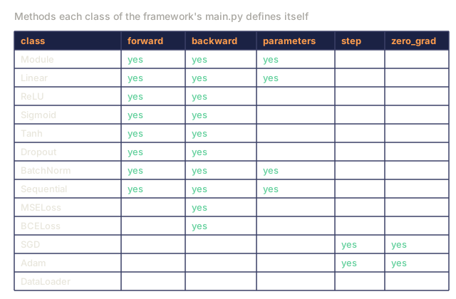
A Module is the base unit of a framework: anything with a forward pass, a backward pass, and a list of trainable parameters. Every layer in PyTorch inherits from nn.Module, and every Module carries the same three responsibilities:

forward(): compute the output given inputs
parameters(): return all trainable weights
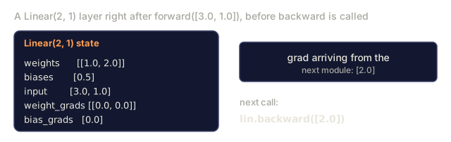
backward(): compute gradients (handled by autograd in PyTorch, explicit in ours)

A Linear layer is a Module. So is a ReLU activation, a dropout layer, a batch normalization layer. Four different jobs, one interface.

Sequential Container

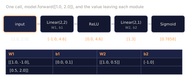
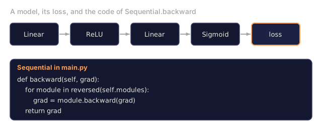
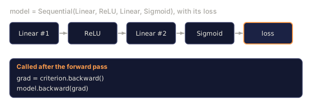
nn.Sequential chains Modules. Forward pass: feed data through Module 1, then Module 2, then Module 3. Backward pass: reverse the chain. The container itself is a Module: it has forward(), parameters(), and backward(). This is the composite pattern: a sequence of Modules is itself a Module.

Training vs Evaluation Mode

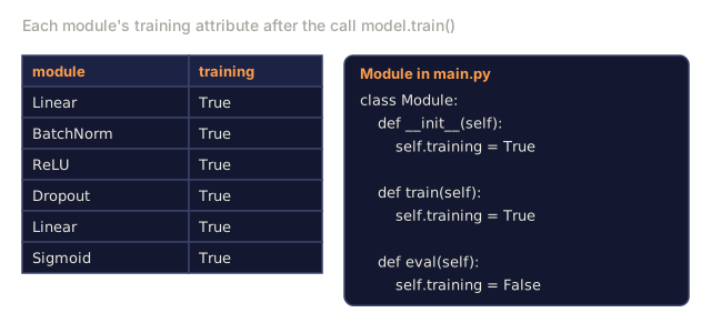
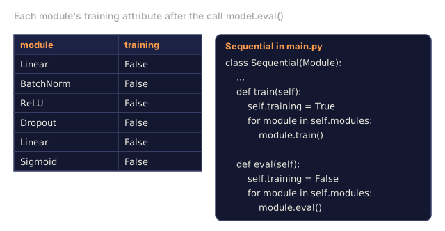
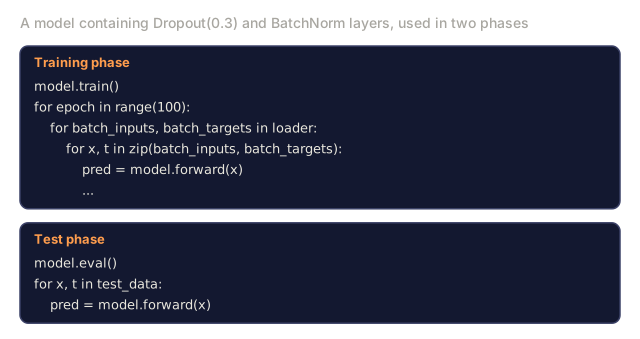
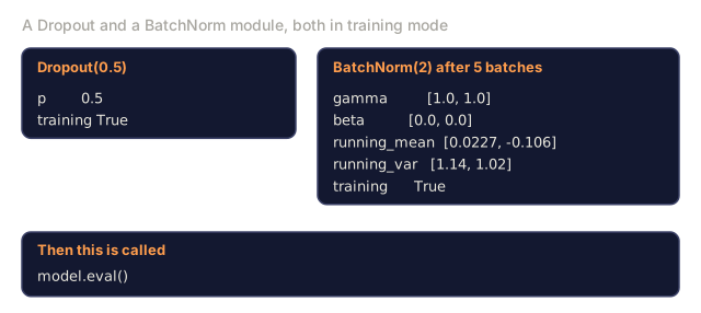
Dropout randomly zeroes neurons during training but passes everything through during evaluation. Batch normalization uses batch statistics during training but running averages during evaluation. The train() and eval() methods toggle this behavior. Every Module has a training flag.

Optimizer

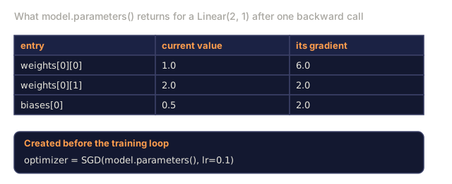
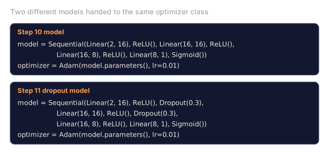
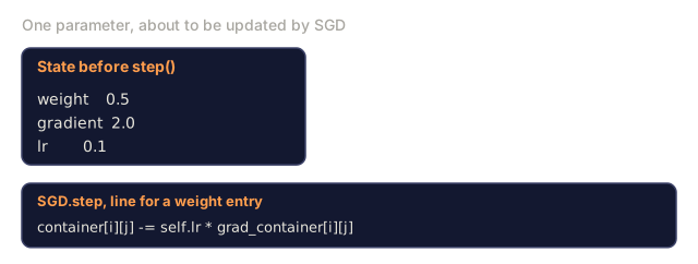
The optimizer updates parameters using their gradients. SGD: param -= lr * grad. Adam: maintains momentum and variance estimates, then updates. The optimizer doesn't know anything about the network architecture. It only sees a flat list of parameters and their gradients.

DataLoader

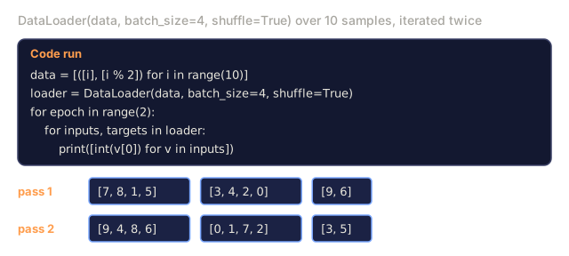
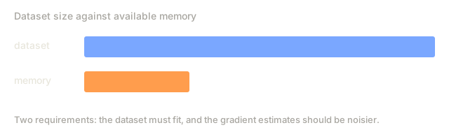
Batching matters for two reasons. First, you cannot fit the entire dataset in memory for large problems. Second, mini-batch gradient descent provides noise that helps escape local minima. The DataLoader splits data into batches and optionally shuffles between epochs.

Framework Architecture

Mermaid diagram

Training Loop

Mermaid diagram

Module Hierarchy

Mermaid diagram

Check: The Concept0/15

1. What is a Module in a deep learning framework, and what three responsibilities does it carry?Define

A tree with the box Module on the left joined by a vertical line to seven boxes in a column: Linear, ReLU, Sigmoid, Tanh, Dropout, BatchNorm and Sequential, each written with (Module), followed by one line of code that builds a Sequential from Linear, ReLU and Sigmoid objects. — The seven classes are read from main.py with Module.__subclasses__().

2. What is a Sequential container?Define

A dashed outer box labelled Sequential containing eight inner boxes in two rows: Linear 2 to 16, ReLU, Linear 16 to 16, ReLU, Linear 16 to 8, ReLU, Linear 8 to 1, Sigmoid. — Layer sizes as in the lesson's Step 10.

3. What does the forward pass do?Define

A chain of five boxes, the input [1.0, 2.0], Linear(2,2), ReLU, Linear(2,1) and Sigmoid, each with the value leaving it printed below: [-1.0, 4.6], [0.0, 4.6], [1.3] and [0.7858]. A table lists the weights and biases of the two Linear layers. — Weights typed by hand (illustrative); every value was produced by calling the lesson's classes.

4. What does the backward pass produce?Define

A card with the state of a Linear(2,1) layer after forward on [3.0, 1.0]: weights [[1.0, 2.0]], bias [0.5], cached input [3.0, 1.0] and all-zero gradient buffers, next to a box saying the gradient arriving from the next module is [2.0] and the next call is lin.backward([2.0]). — State read from the lesson's Linear class (weights set by hand).

5. In this framework, what counts as a parameter?Define

Three cards: a Linear(2,3) layer listing its weights, biases, zero gradient buffers and cached input; a ReLU holding the mask [1.0, 0.0, 1.0] for the Linear output [5.5, -1.0, 1.0]; and the two constructor calls Adam with lr=0.01 and DataLoader with batch_size=16. — Linear and ReLU fields read from the lesson's classes (weights set by hand).

6. What is training mode?Define

A table listing six modules of a Sequential model, Linear, BatchNorm, ReLU, Dropout, Linear and Sigmoid, each with training equal to True after model.train(), next to the Module base class source with its training attribute and its train and eval methods. — Table read from a real model; code copied from main.py.

7. What is evaluation mode?Define

A table listing six modules of a Sequential model, Linear, BatchNorm, ReLU, Dropout, Linear and Sigmoid, each with training equal to False after model.eval(), next to the train and eval methods of Sequential from main.py. — Table read from a real model; code copied from main.py.

8. What is the job of an optimizer?Define

A table of the three parameter entries of a Linear(2,1) layer after one backward call: weights[0][0] value 1.0 gradient 6.0, weights[0][1] value 2.0 gradient 2.0 and biases[0] value 0.5 gradient 2.0, above the line optimizer = SGD(model.parameters(), lr=0.1). — Values read from the lesson's Linear.parameters().

9. What is the role of the DataLoader in the framework?Define

The code that builds a DataLoader over ten samples with batch_size 4 and shuffle True and loops over it twice, followed by the batches printed for each pass as lists of sample numbers. — Batches captured from running the lesson's DataLoader with random.seed(0).

10. Why does Sequential run its modules in reverse order during the backward pass?Explain

A chain of boxes Linear, ReLU, Linear, Sigmoid and loss joined by arrows, above the source of Sequential.backward: a loop over reversed(self.modules) that calls module.backward(grad). — Code read from main.py.

11. Why does a framework need separate train and eval modes?Explain

Two code boxes. The training phase calls model.train() and loops over epochs, batches and samples calling model.forward(x). The test phase calls model.eval() and loops over test_data calling model.forward(x). — Shortened from the lesson's Step 10 and Step 11 loops.

12. How does the optimizer relate to the network's architecture?Explain

Two code boxes. The Step 10 model is a Sequential of Linear and ReLU layers ending in Sigmoid, and the Step 11 model adds two Dropout(0.3) layers. Both are followed by the same line creating Adam(model.parameters(), lr=0.01). — Model definitions copied from the lesson.

13. You add a custom layer that injects noise only during training and has no weights. What must it do for Sequential and the optimizer to work unchanged?Design

A code box with an empty NoiseLayer class that inherits from Module, a model definition with a NoiseLayer between ReLU and the second Linear, and an Adam optimizer on model.parameters(). — NoiseLayer is hypothetical; its body is left out.

14. You want L2 weight decay applied to every parameter, whatever the architecture. Where does it belong?Design

Five boxes for a model with a Linear(2,4) holding weights and biases (12 entries), a BatchNorm(4) holding gamma and beta (8 entries), a ReLU with none, a Linear(4,1) holding weights and biases (5 entries) and a Sigmoid with none. — Entry counts read from the lesson's classes; the model is an example.

15. Your dataset has grown too large to fit in memory, and you also want noisier gradient estimates. Which part of the framework addresses both?Design

Two horizontal bars: a long bar for the dataset and a much shorter bar for the memory available, with a note listing two requirements: the dataset must fit, and the gradient estimates should be noisier. — Illustrative bars, not measured and not to scale; no real sizes are implied.

Build It

Step 1: Module Base Class

The abstract interface that every layer implements.

python

class Module:
    def __init__(self):
        self.training = True
 
    def forward(self, x):
        raise NotImplementedError
 
    def backward(self, grad):
        raise NotImplementedError
 
    def parameters(self):
        return []
 
    def train(self):
        self.training = True
 
    def eval(self):
        self.training = False

Step 2: Linear Layer

The fundamental building block. Stores weights and biases, computes Wx + b forward, and weight/input gradients backward.

python

import math
import random
 
 
class Linear(Module):
    def __init__(self, fan_in, fan_out):
        super().__init__()
        std = math.sqrt(2.0 / fan_in)
        self.weights = [[random.gauss(0, std) for _ in range(fan_in)] for _ in range(fan_out)]
        self.biases = [0.0] * fan_out
        self.weight_grads = [[0.0] * fan_in for _ in range(fan_out)]
        self.bias_grads = [0.0] * fan_out
        self.fan_in = fan_in
        self.fan_out = fan_out
        self.input = None
 
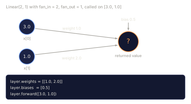
    def forward(self, x):
        self.input = x
        output = []
        for i in range(self.fan_out):
            val = self.biases[i]
            for j in range(self.fan_in):
                val += self.weights[i][j] * x[j]
            output.append(val)
        return output
 
    def backward(self, grad):
        input_grad = [0.0] * self.fan_in
        for i in range(self.fan_out):
            self.bias_grads[i] += grad[i]
            for j in range(self.fan_in):
                self.weight_grads[i][j] += grad[i] * self.input[j]
                input_grad[j] += grad[i] * self.weights[i][j]
        return input_grad
 
    def parameters(self):
        params = []
        for i in range(self.fan_out):
            for j in range(self.fan_in):
                params.append((self.weights, i, j, self.weight_grads))
            params.append((self.biases, i, None, self.bias_grads))
        return params

Step 3: Activation Modules

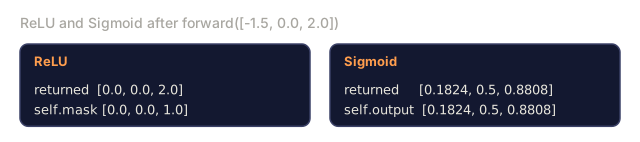
ReLU, Sigmoid, and Tanh as Modules. Each caches what it needs for the backward pass.

python

class ReLU(Module):
    def __init__(self):
        super().__init__()
        self.mask = None
 
    def forward(self, x):
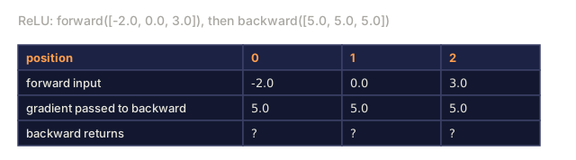
        self.mask = [1.0 if v > 0 else 0.0 for v in x]
        return [max(0.0, v) for v in x]
 
    def backward(self, grad):
        return [g * m for g, m in zip(grad, self.mask)]
 
 
class Sigmoid(Module):
    def __init__(self):
        super().__init__()
        self.output = None
 
    def forward(self, x):
        self.output = []
        for v in x:
            v = max(-500, min(500, v))
            self.output.append(1.0 / (1.0 + math.exp(-v)))
        return self.output
 
    def backward(self, grad):
        return [g * o * (1 - o) for g, o in zip(grad, self.output)]
 
 
class Tanh(Module):
    def __init__(self):
        super().__init__()
        self.output = None
 
    def forward(self, x):
        self.output = [math.tanh(v) for v in x]
        return self.output
 
    def backward(self, grad):
        return [g * (1 - o * o) for g, o in zip(grad, self.output)]

Step 4: Dropout Module

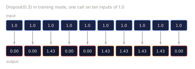
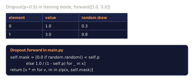
Randomly zeroes elements during training. Scales remaining elements by 1/(1-p) so expected values stay the same. Does nothing during eval.

python

class Dropout(Module):
    def __init__(self, p=0.5):
        super().__init__()
        self.p = p
        self.mask = None
 
    def forward(self, x):
        if not self.training:
            return x
        self.mask = [0.0 if random.random() < self.p else 1.0 / (1 - self.p) for _ in x]
        return [v * m for v, m in zip(x, self.mask)]
 
    def backward(self, grad):
        if self.mask is None:
            return grad
        return [g * m for g, m in zip(grad, self.mask)]

Step 5: BatchNorm Module

Normalizes activations to zero mean and unit variance per feature across the batch. Maintains running statistics for eval mode.

python

class BatchNorm(Module):
    def __init__(self, size, momentum=0.1, eps=1e-5):
        super().__init__()
        self.size = size
        self.gamma = [1.0] * size
        self.beta = [0.0] * size
        self.gamma_grads = [0.0] * size
        self.beta_grads = [0.0] * size
        self.running_mean = [0.0] * size
        self.running_var = [1.0] * size
        self.momentum = momentum
        self.eps = eps
        self.x_norm = None
        self.std_inv = None
        self.batch_input = None
 
    def forward_batch(self, batch):
        batch_size = len(batch)
        output_batch = []
 
        if self.training:
            mean = [0.0] * self.size
            for sample in batch:
                for j in range(self.size):
                    mean[j] += sample[j]
            mean = [m / batch_size for m in mean]
 
            var = [0.0] * self.size
            for sample in batch:
                for j in range(self.size):
                    var[j] += (sample[j] - mean[j]) ** 2
            var = [v / batch_size for v in var]
 
            self.std_inv = [1.0 / math.sqrt(v + self.eps) for v in var]
 
            self.x_norm = []
            self.batch_input = batch
            for sample in batch:
                normed = [(sample[j] - mean[j]) * self.std_inv[j] for j in range(self.size)]
                self.x_norm.append(normed)
                output = [self.gamma[j] * normed[j] + self.beta[j] for j in range(self.size)]
                output_batch.append(output)
 
            for j in range(self.size):
                self.running_mean[j] = (1 - self.momentum) * self.running_mean[j] + self.momentum * mean[j]
                self.running_var[j] = (1 - self.momentum) * self.running_var[j] + self.momentum * var[j]
        else:
            std_inv = [1.0 / math.sqrt(v + self.eps) for v in self.running_var]
            for sample in batch:
                normed = [(sample[j] - self.running_mean[j]) * std_inv[j] for j in range(self.size)]
                output = [self.gamma[j] * normed[j] + self.beta[j] for j in range(self.size)]
                output_batch.append(output)
 
        return output_batch
 
    def forward(self, x):
        result = self.forward_batch([x])
        return result[0]
 
    def backward(self, grad):
        if self.x_norm is None:
            return grad
        for j in range(self.size):
            self.gamma_grads[j] += self.x_norm[0][j] * grad[j]
            self.beta_grads[j] += grad[j]
        return [grad[j] * self.gamma[j] * self.std_inv[j] for j in range(self.size)]
 
    def parameters(self):
        params = []
        for j in range(self.size):
            params.append((self.gamma, j, None, self.gamma_grads))
            params.append((self.beta, j, None, self.beta_grads))
        return params

Step 6: Sequential Container

Chains modules. Forward goes left-to-right, backward goes right-to-left.

python

class Sequential(Module):
    def __init__(self, *modules):
        super().__init__()
        self.modules = list(modules)
 
    def forward(self, x):
        for module in self.modules:
            x = module.forward(x)
        return x
 
    def backward(self, grad):
        for module in reversed(self.modules):
            grad = module.backward(grad)
        return grad
 
    def parameters(self):
        params = []
        for module in self.modules:
            params.extend(module.parameters())
        return params
 
    def train(self):
        self.training = True
        for module in self.modules:
            module.train()
 
    def eval(self):
        self.training = False
        for module in self.modules:
            module.eval()

Step 7: Loss Functions

MSE and Binary Cross-Entropy. Each returns the loss value and provides a backward() that returns the gradient.

python

class MSELoss:
    def __call__(self, predicted, target):
        self.predicted = predicted
        self.target = target
        n = len(predicted)
        self.loss = sum((p - t) ** 2 for p, t in zip(predicted, target)) / n
        return self.loss
 
    def backward(self):
        n = len(self.predicted)
        return [2 * (p - t) / n for p, t in zip(self.predicted, self.target)]
 
 
class BCELoss:
    def __call__(self, predicted, target):
        self.predicted = predicted
        self.target = target
        eps = 1e-7
        n = len(predicted)
        self.loss = 0
        for p, t in zip(predicted, target):
            p = max(eps, min(1 - eps, p))
            self.loss += -(t * math.log(p) + (1 - t) * math.log(1 - p))
        self.loss /= n
        return self.loss
 
    def backward(self):
        eps = 1e-7
        n = len(self.predicted)
        grads = []
        for p, t in zip(self.predicted, self.target):
            p = max(eps, min(1 - eps, p))
            grads.append((-t / p + (1 - t) / (1 - p)) / n)
        return grads

Step 8: SGD and Adam Optimizers

Both take a parameter list and update weights using gradients.

python

class SGD:
    def __init__(self, parameters, lr=0.01):
        self.params = parameters
        self.lr = lr
 
    def step(self):
        for container, i, j, grad_container in self.params:
            if j is not None:
                container[i][j] -= self.lr * grad_container[i][j]
            else:
                container[i] -= self.lr * grad_container[i]
 
    def zero_grad(self):
        for container, i, j, grad_container in self.params:
            if j is not None:
                grad_container[i][j] = 0.0
            else:
                grad_container[i] = 0.0
 
 
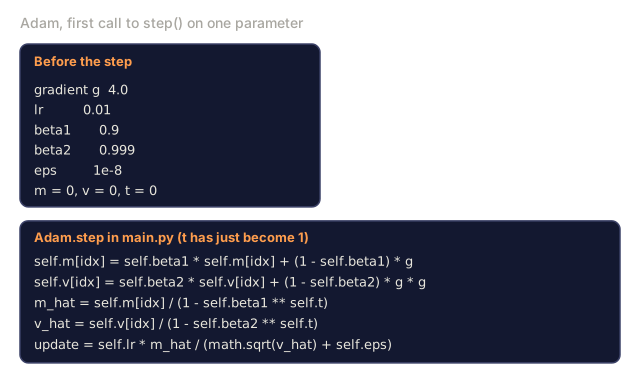
class Adam:
    def __init__(self, parameters, lr=0.001, beta1=0.9, beta2=0.999, eps=1e-8):
        self.params = parameters
        self.lr = lr
        self.beta1 = beta1
        self.beta2 = beta2
        self.eps = eps
        self.t = 0
        self.m = [0.0] * len(parameters)
        self.v = [0.0] * len(parameters)
 
    def step(self):
        self.t += 1
        for idx, (container, i, j, grad_container) in enumerate(self.params):
            if j is not None:
                g = grad_container[i][j]
            else:
                g = grad_container[i]
 
            self.m[idx] = self.beta1 * self.m[idx] + (1 - self.beta1) * g
            self.v[idx] = self.beta2 * self.v[idx] + (1 - self.beta2) * g * g
 
            m_hat = self.m[idx] / (1 - self.beta1 ** self.t)
            v_hat = self.v[idx] / (1 - self.beta2 ** self.t)
 
            update = self.lr * m_hat / (math.sqrt(v_hat) + self.eps)
 
            if j is not None:
                container[i][j] -= update
            else:
                container[i] -= update
 
    def zero_grad(self):
        for container, i, j, grad_container in self.params:
            if j is not None:
                grad_container[i][j] = 0.0
            else:
                grad_container[i] = 0.0

Step 9: DataLoader

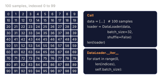
Splits data into batches, optionally shuffles each epoch.

python

class DataLoader:
    def __init__(self, data, batch_size=32, shuffle=True):
        self.data = data
        self.batch_size = batch_size
        self.shuffle = shuffle
 
    def __iter__(self):
        indices = list(range(len(self.data)))
        if self.shuffle:
            random.shuffle(indices)
        for start in range(0, len(indices), self.batch_size):
            batch_indices = indices[start:start + self.batch_size]
            batch = [self.data[i] for i in batch_indices]
            inputs = [item[0] for item in batch]
            targets = [item[1] for item in batch]
            yield inputs, targets
 
    def __len__(self):
        return (len(self.data) + self.batch_size - 1) // self.batch_size

Step 10: Train a 4-Layer Network on Circle Classification

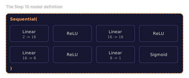
Wire everything together. Define a model, pick a loss, pick an optimizer, run the training loop.

python

def make_circle_data(n=500, seed=42):
    random.seed(seed)
    data = []
    for _ in range(n):
        x = random.uniform(-2, 2)
        y = random.uniform(-2, 2)
        label = 1.0 if x * x + y * y < 1.5 else 0.0
        data.append(([x, y], [label]))
    return data
 
 
def train_framework():
    random.seed(42)
 
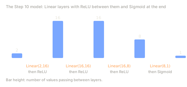
    model = Sequential(
        Linear(2, 16),
        ReLU(),
        Linear(16, 16),
        ReLU(),
        Linear(16, 8),
        ReLU(),
        Linear(8, 1),
        Sigmoid(),
    )
 
    criterion = BCELoss()
    optimizer = Adam(model.parameters(), lr=0.01)
 
    data = make_circle_data(500)
    split = int(len(data) * 0.8)
    train_data = data[:split]
    test_data = data[split:]
 
    loader = DataLoader(train_data, batch_size=16, shuffle=True)
 
    model.train()
 
    for epoch in range(100):
        total_loss = 0
        total_correct = 0
        total_samples = 0
 
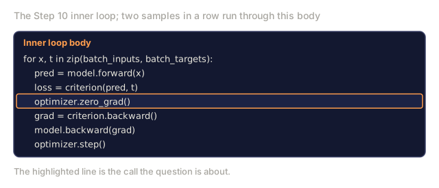
        for batch_inputs, batch_targets in loader:
            batch_loss = 0
            for x, t in zip(batch_inputs, batch_targets):
                pred = model.forward(x)
                loss = criterion(pred, t)
                batch_loss += loss
 
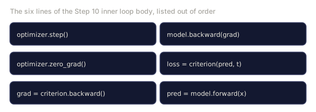
                optimizer.zero_grad()
                grad = criterion.backward()
                model.backward(grad)
                optimizer.step()
 
                predicted_class = 1.0 if pred[0] >= 0.5 else 0.0
                if predicted_class == t[0]:
                    total_correct += 1
                total_samples += 1
 
            total_loss += batch_loss
 
        avg_loss = total_loss / total_samples
        accuracy = total_correct / total_samples * 100
 
        if epoch % 10 == 0 or epoch == 99:
            print(f"Epoch {epoch:3d} | Loss: {avg_loss:.6f} | Train Accuracy: {accuracy:.1f}%")
 
    model.eval()
    correct = 0
    for x, t in test_data:
        pred = model.forward(x)
        predicted_class = 1.0 if pred[0] >= 0.5 else 0.0
        if predicted_class == t[0]:
            correct += 1
    test_accuracy = correct / len(test_data) * 100
    print(f"\nTest Accuracy: {test_accuracy:.1f}% ({correct}/{len(test_data)})")
 
    return model, test_accuracy

Step 11: Train/Eval Mode in Practice

Step 10's network never touches Dropout or BatchNorm, so model.train() and model.eval() only flip a flag that nothing reads. Wire in the two modules that actually check self.training, and the toggle stops being decorative.

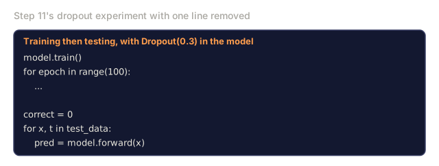
Dropout is the easy case. Insert it between hidden layers, run the same circle-classification loop from Step 10, and switch to model.eval() before the test pass so dropout stops zeroing neurons.

python

def train_with_dropout():
    random.seed(42)
 
    model = Sequential(
        Linear(2, 16),
        ReLU(),
        Dropout(0.3),
        Linear(16, 16),
        ReLU(),
        Dropout(0.3),
        Linear(16, 8),
        ReLU(),
        Linear(8, 1),
        Sigmoid(),
    )
 
    criterion = BCELoss()
    optimizer = Adam(model.parameters(), lr=0.01)
 
    data = make_circle_data(500)
    split = int(len(data) * 0.8)
    train_data = data[:split]
    test_data = data[split:]
    loader = DataLoader(train_data, batch_size=16, shuffle=True)
 
    model.train()
 
    for epoch in range(100):
        for batch_inputs, batch_targets in loader:
            for x, t in zip(batch_inputs, batch_targets):
                pred = model.forward(x)
                criterion(pred, t)
                optimizer.zero_grad()
                grad = criterion.backward()
                model.backward(grad)
                optimizer.step()
 
    model.eval()
    correct = 0
    for x, t in test_data:
        pred = model.forward(x)
        predicted_class = 1.0 if pred[0] >= 0.5 else 0.0
        if predicted_class == t[0]:
            correct += 1
    return correct / len(test_data) * 100

Run it and test accuracy comes back at 98.0%, against 97.0% for the identical architecture with no dropout at all. Dropout barely moves the number on a network this small, but the mechanism, zero neurons during training and pass everything through during eval, is now something you watched happen instead of something you read about.

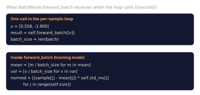
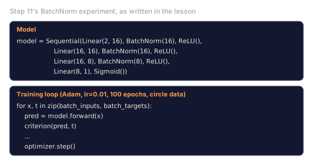
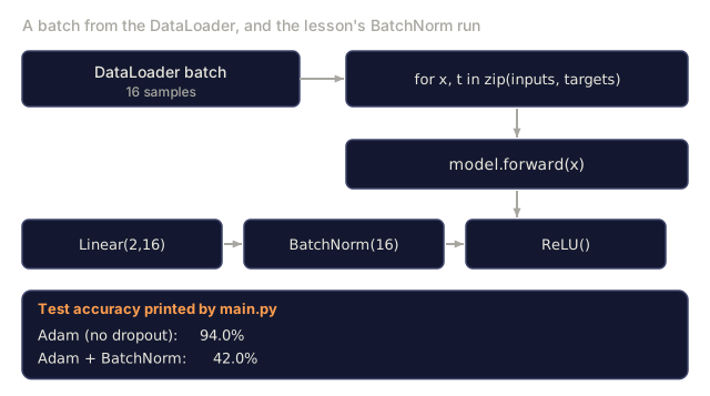
Now try BatchNorm, and remember Lesson 07: batch normalization depends on batch statistics, and at batch size 1 those statistics are meaningless. This framework's Module.forward() takes exactly one sample at a time, everywhere, by the contract Step 1 set. Drop BatchNorm into the Sequential and every one of its forward_batch([x]) calls runs on a batch of exactly one element.

python

def train_with_batchnorm():
    random.seed(42)
 
    model = Sequential(
        Linear(2, 16),
        BatchNorm(16),
        ReLU(),
        Linear(16, 16),
        BatchNorm(16),
        ReLU(),
        Linear(16, 8),
        BatchNorm(8),
        ReLU(),
        Linear(8, 1),
        Sigmoid(),
    )
 
    criterion = BCELoss()
    optimizer = Adam(model.parameters(), lr=0.01)
 
    data = make_circle_data(500)
    split = int(len(data) * 0.8)
    train_data = data[:split]
    test_data = data[split:]
    loader = DataLoader(train_data, batch_size=16, shuffle=True)
 
    model.train()
 
    for epoch in range(100):
        for batch_inputs, batch_targets in loader:
            for x, t in zip(batch_inputs, batch_targets):
                pred = model.forward(x)
                criterion(pred, t)
                optimizer.zero_grad()
                grad = criterion.backward()
                model.backward(grad)
                optimizer.step()
 
    first_bn = model.modules[1]
    print(f"After training, first BatchNorm layer: running_var[0] = {first_bn.running_var[0]:.10f}")
 
    model.eval()
    correct = 0
    for x, t in test_data:
        pred = model.forward(x)
        predicted_class = 1.0 if pred[0] >= 0.5 else 0.0
        if predicted_class == t[0]:
            correct += 1
    return correct / len(test_data) * 100

Run this one and test accuracy collapses to 42.0%, on the same data, same optimizer, same 100 epochs that got 97-98% everywhere else. Check running_var[0] on the first BatchNorm layer after training and it has decayed to 0.0000000000.

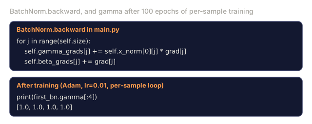
The mean of a one-element batch is that element, so the variance is always exactly zero, so x_norm is always exactly zero, on every single call. output = gamma * x_norm + beta collapses to output = beta, a constant that never depends on the input. It gets worse on the way back: gamma_grads[j] += x_norm[j] * grad[j] multiplies by that same always-zero x_norm, so gamma never receives a gradient and stays at its initial value of 1.0 forever. Only beta learns anything, and a single learned offset per feature can't encode what the input actually was. Every BatchNorm layer becomes a hole punched through the network: whatever the layers before it computed, the layers after it never see it.

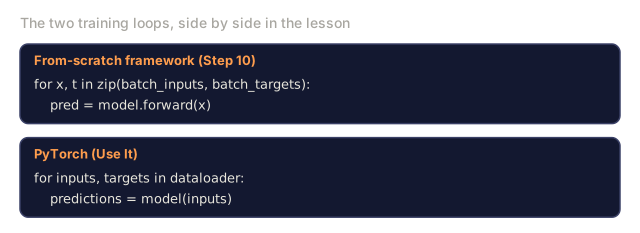
This isn't a typo-level bug. It's what happens when a module written to expect real batch statistics gets called one sample at a time. PyTorch's nn.Module.forward() never runs into this because every tensor carries a real batch dimension end to end, so nn.BatchNorm1d sees the same 16, 32, or 64 samples your DataLoader assembled, not one. Fixing it here means making Sequential.forward() batch-shaped from input to output, not just handing BatchNorm its own private multi-sample call. Exercise 6 asks you to do exactly that.

Check: Build It0/22

1. What does zero_grad do?Define

A card showing a Linear(2,1) layer after backward with weights [[1.0, 2.0]], bias [0.5], cached input [3.0, 1.0], gradients [[6.0, 2.0]] and [2.0] and learning rate 0.1, beside the two code lines model.backward(grad) and optimizer.zero_grad() with the second highlighted as the next to run. — State from the lesson's classes with an SGD optimizer at lr=0.1.

2. Why does the training loop need an explicit zero_grad() call before each backward pass?Explain

The seven lines of the Step 10 inner loop: forward, loss, optimizer.zero_grad(), criterion.backward(), model.backward(grad) and optimizer.step(), with the optimizer.zero_grad() line highlighted. — Copied from Step 10.

3. In the Dropout and BatchNorm code, what changes between training and eval mode?Explain

Two cards: Dropout(0.5) with training True, and BatchNorm(2) after five training batches with gamma [1.0, 1.0], beta [0.0, 0.0], running_mean [0.0227, -0.106], running_var [1.14, 1.02] and training True, above the line model.eval(). — BatchNorm state captured after five forward_batch calls on 8 points each of the lesson's circle data.

4. Why does Dropout scale the surviving elements by 1/(1-p) during training?Explain

A row of ten input cells each 1.0, arrows down to ten output cells: 5 of them are 0.00 and the rest are 1.43. — p = 0.3 as in Step 11; one random draw from the lesson's Dropout (seed 4).

5. Why do ReLU and Sigmoid store a mask or their output during forward()?Explain

Two cards after forward on [-1.5, 0.0, 2.0]: ReLU returned [0.0, 0.0, 2.0] and holds the attribute mask [0.0, 0.0, 1.0]; Sigmoid returned [0.1824, 0.5, 0.8808] and holds the same values in the attribute output. — Values read from the lesson's ReLU and Sigmoid.

6. What happens to the statistics batch normalization relies on when every batch contains a single sample?Explain

Two code boxes: a call forward_batch([x]) with x = [0.558, -1.900], the first circle sample, and the lines of forward_batch that divide the sums by batch_size and normalize each sample. — x is the first point of the lesson's make_circle_data(500).

7. Which design choice in PyTorch avoids the mini framework's BatchNorm failure entirely?Explain

Two code boxes. The from-scratch loop zips batch_inputs with batch_targets and calls model.forward(x) per pair; the PyTorch loop iterates a dataloader and calls model(inputs). — Both snippets copied from the lesson.

8. In the Step 10 training loop, what is the order of calls for each sample?Apply

Six cards in a 2 by 3 grid, each holding one line of the Step 10 inner loop in scrambled order: optimizer.step(), model.backward(grad), optimizer.zero_grad(), loss = criterion(pred, t), grad = criterion.backward() and pred = model.forward(x). — Lines copied from Step 10; the order shown is not the loop's order.

9. A Linear layer has fan_in = 2, fan_out = 1, weights [[1.0, 2.0]] and biases [0.5]. What does forward([3.0, 1.0]) return?Apply

A diagram of a Linear layer with two inputs 3.0 and 1.0, connection weights 1.0 and 2.0, a bias of 0.5 and an output marked with a question mark, above the three code lines that set weights [[1.0, 2.0]], biases [0.5] and call forward([3.0, 1.0]).

10. A ReLU module runs forward([-2.0, 0.0, 3.0]). Then backward([5.0, 5.0, 5.0]) is called. What does backward return?Apply

A table with positions 0, 1 and 2: the forward input is -2.0, 0.0 and 3.0, the gradient passed to backward is 5.0 in each position, and the row for what backward returns is filled with question marks.

11. A Dropout(p=0.5) layer in training mode gets input [1.0, 3.0]. The two random draws are 0.3 and then 0.8. What does forward return?Apply

A table of two elements, value 1.0 with random draw 0.3 and value 3.0 with random draw 0.8, above the Dropout.forward lines that build the mask from random.random() < self.p and multiply the input by it. — Code copied from main.py.

12. A DataLoader wraps 100 samples with batch_size=32 and shuffle=False. What does len(loader) return, and how big is the last batch?Apply

Code copied from main.py.

13. An SGD optimizer with lr=0.1 steps on a weight of 0.5 whose gradient is 2.0. What is the weight afterwards?Apply

A card with a weight of 0.5, a gradient of 2.0 and learning rate 0.1, above the line from SGD.step: container[i][j] -= self.lr * grad_container[i][j]. — Update line copied from main.py.

14. Adam with lr=0.01 and the default betas takes its first step (t=1) on a weight whose gradient is 4.0. About how much does the weight decrease?Apply

A card listing the start of an Adam step: gradient 4.0, lr 0.01, beta1 0.9, beta2 0.999, eps 1e-8 and m, v and t all zero, above the five lines of Adam.step that update m, update v, correct both and compute the update. — Update lines copied from main.py.

15. A model is Sequential(Linear, ReLU, Linear, Sigmoid). When backward(grad) is called with the loss gradient, which module's backward runs first and what does it receive?Apply

A chain of boxes Linear #1, ReLU, Linear #2, Sigmoid and loss joined by arrows, above the two code lines grad = criterion.backward() and model.backward(grad).

16. The Step 10 model is Linear(2,16), Linear(16,16), Linear(16,8), Linear(8,1) with activations between them. How many entries does model.parameters() return?Apply

Five bars showing the number of values entering and leaving the Linear layers of the Step 10 model: 2, 16, 16, 8 and 1, labelled Linear(2,16), Linear(16,16), Linear(16,8) and Linear(8,1) with ReLU after the first three and Sigmoid after the last. — Layer sizes from the lesson's Step 10.

17. BatchNorm layers are added to the Sequential model and trained with the per-sample loop. What does the lesson's run show?Analyze

Two code boxes from Step 11: a Sequential with a BatchNorm after each of the first three Linear layers, and the per-sample training loop that calls model.forward(x) and optimizer.step() for each sample. — Shortened from the lesson's train_with_batchnorm.

18. A loop runs forward, loss, backward, then optimizer.zero_grad(), then optimizer.step(). What does training do?Analyze

A setup card (Linear(2,1) with weights [[1.0, 2.0]], bias [0.5], input [3.0, 1.0], target [5.0], MSELoss and SGD with lr 0.1) above a six-line loop body in the order forward, loss, criterion.backward, model.backward, optimizer.zero_grad, optimizer.step, with the last two lines highlighted. — Setup values are illustrative; the loop order is the one in the question.

19. A model with Dropout layers is trained, then the test loop runs without calling model.eval(). What symptom should you expect?Analyze

A code box with model.train(), the epoch loop elided, and then a test loop over test_data calling model.forward(x); there is no model.eval() line anywhere. — Edited copy of Step 11: the model.eval() line is deleted.

20. After per-sample training with BatchNorm, gamma is still exactly 1.0. Which explanation matches the code?Analyze

The gradient lines of BatchNorm.backward, which add x_norm[0][j] * grad[j] to gamma_grads and grad[j] to beta_grads, above the printed first four gamma values after training: [1.0, 1.0, 1.0, 1.0]. — Code copied from main.py; gamma printed from a real run of the lesson's Step 11 BatchNorm experiment.

21. In Step 10, optimizer.step() runs after every sample inside each batch of 16. What does batch_size=16 actually change in this loop?Analyze

The Step 10 training code: a DataLoader over train_data with batch_size=16 and shuffle=True, an outer loop over batches, an inner loop over the samples of a batch, and in the inner loop forward, loss, zero_grad, criterion.backward, model.backward and optimizer.step. — Code copied from Step 10; the training set has 400 samples (500, 80/20 split).

22. You want BatchNorm to work in this framework. Which change addresses the root cause?Design

A flow: a DataLoader batch of 16 samples goes into a loop over x and t, then model.forward(x), through Linear(2,16), BatchNorm(16) and ReLU(). Below, two lines of main.py output: Adam without dropout 94.0% and Adam with BatchNorm 42.0%. — Structure of the lesson's Step 10 and Step 11 code; the two output lines come from running main.py.

Use It

Here is the PyTorch equivalent of what you just built:

python

import torch
import torch.nn as nn
from torch.utils.data import DataLoader, TensorDataset
 
model = nn.Sequential(
    nn.Linear(2, 16),
    nn.ReLU(),
    nn.Linear(16, 16),
    nn.ReLU(),
    nn.Linear(16, 8),
    nn.ReLU(),
    nn.Linear(8, 1),
    nn.Sigmoid(),
)
 
criterion = nn.BCELoss()
optimizer = torch.optim.Adam(model.parameters(), lr=0.01)
 
for epoch in range(100):
    model.train()
    for inputs, targets in dataloader:
        optimizer.zero_grad()
        predictions = model(inputs)
        loss = criterion(predictions, targets)
        loss.backward()
        optimizer.step()
 
    model.eval()
    with torch.no_grad():
        test_predictions = model(test_inputs)

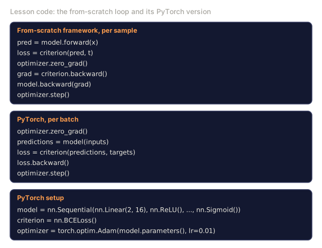
The structure is identical: Sequential, Linear, ReLU, Sigmoid, BCELoss, Adam, zero_grad, backward, step, train, eval. Every concept maps one-to-one. PyTorch's version handles autograd automatically (no need to implement backward() in each module), runs on GPU, and has years of optimization behind it, but the bones are the same.

Now when you see PyTorch code, you know exactly what's happening at every line. That understanding is the whole point.

Check: Use It0/2

1. Which part of the from-scratch framework does the PyTorch version let you skip writing?Explain

A table with one row per class of main.py (Module, Linear, ReLU, Sigmoid, Tanh, Dropout, BatchNorm, Sequential, MSELoss, BCELoss, SGD, Adam, DataLoader) and columns forward, backward, parameters, step and zero_grad, with yes where the class defines that method itself. 10 classes define backward. — Read from main.py with inspect; a blank means the class does not define that method.

2. How does the PyTorch training code compare with the from-scratch framework's structure?Explain

Three code boxes copied from the lesson: the from-scratch per-sample loop body, the PyTorch per-batch loop body, and the PyTorch setup lines creating nn.Sequential, nn.BCELoss and Adam. — Snippets copied from Step 10 and the Use It section (setup line shortened).

Ship It

This lesson produces:

outputs/prompt-framework-architect.md, a prompt for designing neural network architectures using framework abstractions

Author's Note

The moment that made this lesson worth writing wasn't wiring together ten lessons of pieces. It was watching BatchNorm's test accuracy fall to 42% the first time I actually ran it inside this framework. The module itself was correct: forward_batch() computes real batch mean and variance, exactly like the Concept section describes. The problem was one layer up. Every Module here, including Sequential, passes one sample through forward() at a time, and BatchNorm needs more than one sample to mean anything.

That's not a bug I planted. It's what happens when a design decision made on Step 1, one sample per forward call, because it made every other Module simpler to write, collides with a module that has a real dependency on batch size. PyTorch doesn't hit this because it never made that decision: every tensor carries a batch dimension from the first line of code to the last. Framework design is full of choices like this, made early, that quietly decide what's easy and what's broken three modules later. You don't see them until you build the thing yourself.

Exercises

Add a SoftmaxCrossEntropyLoss class for multi-class classification. Softmax the predictions, compute cross-entropy loss, and handle the combined backward pass. Test it on a 3-class spiral dataset.
Implement learning rate scheduling in the optimizer: add a set_lr() method and wire in the cosine schedule from Lesson 09. Train the circle classifier with warmup + cosine and compare to constant LR.
Add a save() and load() method to Sequential that serializes all weights to a JSON file and loads them back. Verify that a loaded model produces the same predictions as the original.
Implement weight decay (L2 regularization) in the Adam optimizer. Add a weight_decay parameter that shrinks weights toward zero each step. Compare training with decay=0 vs decay=0.01.
Replace the per-sample training loop with proper mini-batch gradient accumulation: accumulate gradients across all samples in a batch, then divide by batch size and take one optimizer step. Measure whether this changes convergence speed.
The BatchNorm module computes correct batch statistics in forward_batch(), but the per-sample training loop in Step 10 always calls forward() with one sample, forcing a batch of size 1 every time BatchNorm runs. Rewrite the training loop so Sequential.forward() and Sequential.backward() accept a real batch (a list of samples) end to end, routing BatchNorm through forward_batch() with the full mini-batch instead of one sample at a time. Confirm accuracy recovers to match the no-BatchNorm baseline.

Key Terms

Term	What people say	What it actually means
Module	"A layer"	The base abstraction in a framework -- anything with forward(), backward(), and parameters()
Sequential	"Stack layers in order"	A container that chains modules, applying them in sequence for forward and reverse for backward
Forward pass	"Run the network"	Computing the output by passing input through each module in order
Backward pass	"Compute gradients"	Propagating the loss gradient through each module in reverse to compute parameter gradients
Parameters	"The trainable weights"	All values in the network that the optimizer can update -- weights and biases
Optimizer	"The thing that updates weights"	An algorithm that uses gradients to update parameters, implementing SGD, Adam, or other rules
DataLoader	"The thing that feeds data"	An iterator that splits a dataset into batches, optionally shuffling between epochs
Training mode	"model.train()"	A flag that enables stochastic behavior like dropout and batch normalization with batch stats
Evaluation mode	"model.eval()"	A flag that disables dropout and uses running statistics for batch normalization
Zero grad	"Clear the gradients"	Resetting all parameter gradients to zero before computing the next batch's gradients

Build Your Own Mini Framework

Learning Objectives

The Problem

The Concept

The Module Abstraction

Sequential Container

Training vs Evaluation Mode

Optimizer

DataLoader

Framework Architecture

Training Loop

Module Hierarchy

Build It

Step 1: Module Base Class

Step 2: Linear Layer

Step 3: Activation Modules

Step 4: Dropout Module

Step 5: BatchNorm Module

Step 6: Sequential Container

Step 7: Loss Functions

Step 8: SGD and Adam Optimizers

Step 9: DataLoader

Step 10: Train a 4-Layer Network on Circle Classification

Step 11: Train/Eval Mode in Practice

Use It

Ship It

Exercises

Key Terms

Further Reading

Code

Ships With