Bias-Variance Tradeoff
Every model error traces back to one of three sources: bias, variance, or noise. You only get to control two of them.
Learning Objectives
- Derive the bias-variance decomposition of expected prediction error and explain the role of irreducible noise
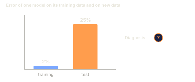
- Diagnose whether a model suffers from high bias or high variance using training and test error patterns
- Explain how regularization techniques (L1, L2, dropout, early stopping) trade bias for variance
- Implement experiments that visualize the bias-variance tradeoff across models of increasing complexity
The Problem
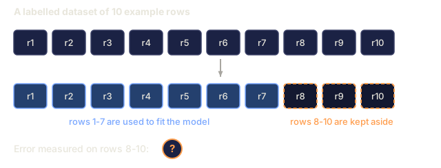
You trained a model. It has some error on the test set. Where did that error come from?
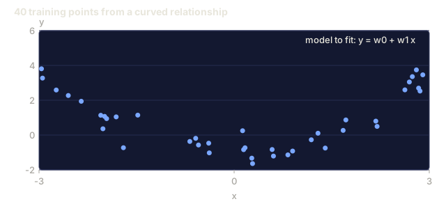
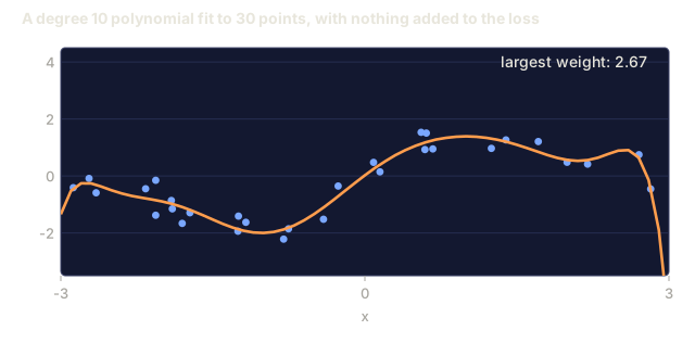
If your model is too simple (linear regression on a curved dataset), it will consistently miss the true pattern. That's bias. If it's too complex (a degree-20 polynomial fit to 15 data points), it will nail the training data and then swing wildly on anything new. That's variance.
You can't push both down at once for a fixed model capacity: push bias down and variance climbs, push variance down and bias climbs. This tradeoff is the most useful diagnostic skill you'll build in machine learning. Once you know which one is hurting you, you know what to do next: make the model more complex or simpler, collect more data or engineer better features, regularize harder or ease off.
The Concept
Bias: Systematic Error
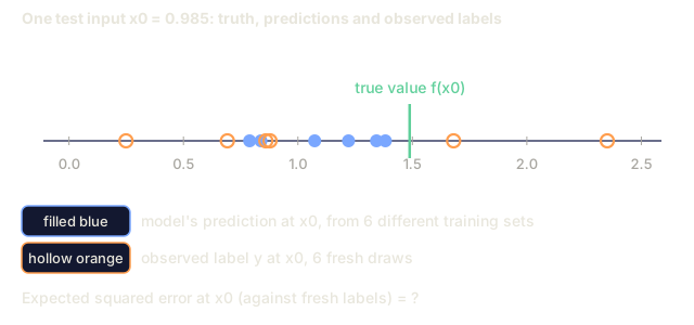
Bias measures how far off your model's average prediction lands from the true value. Train the same model on many different training sets drawn from the same distribution, average the predictions, and bias is the gap between that average and the truth.
High bias means the model is too rigid to capture the real pattern. A straight line fit to a parabola will miss the curve no matter how much data you feed it. That's underfitting.
High bias (underfitting):
  Model always predicts roughly the same wrong thing.
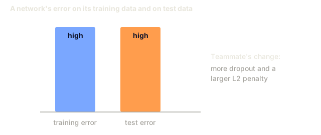
  Training error: HIGH
  Test error: HIGH
  Gap between them: SMALL
Variance: Sensitivity to Training Data
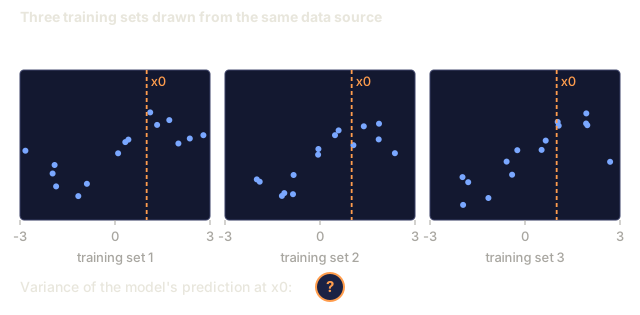
Variance measures how much your predictions swing when you train on different subsets of the same data. Small changes to the training set that cause large changes to the fitted model mean variance is high.
High variance means the model is fitting noise instead of signal. A degree-20 polynomial threads through every training point exactly and oscillates wildly in between. That's overfitting.
High variance (overfitting):
  Model fits training data perfectly but fails on new data.
  Training error: LOW
  Test error: HIGH
  Gap between them: LARGE
The Decomposition
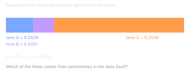
For any point x, expected prediction error under squared loss decomposes exactly into three terms:
Expected Error = Bias^2 + Variance + Irreducible Noise

where:
  Bias^2   = (E[f_hat(x)] - f(x))^2
  Variance = E[(f_hat(x) - E[f_hat(x)])^2]
  Noise    = E[(y - f(x))^2]             (sigma^2)
f(x)is the true functionf_hat(x)is your model's predictionE[...]is the expectation over different training setsyis the observed label (true function plus noise)
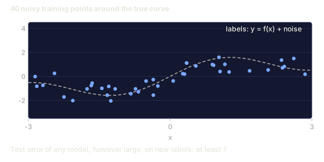
The noise term is irreducible: no model beats sigma^2 on noisy data. Your job is finding the right balance between bias^2 and variance.
Model Complexity vs Error

The classic U-shaped curve:
| Complexity | Bias | Variance | Total Error |
|---|---|---|---|
| Too low | HIGH | LOW | HIGH (underfitting) |
| Just right | MODERATE | MODERATE | LOWEST |
| Too high | LOW | HIGH | HIGH (overfitting) |
Regularization as Bias-Variance Control
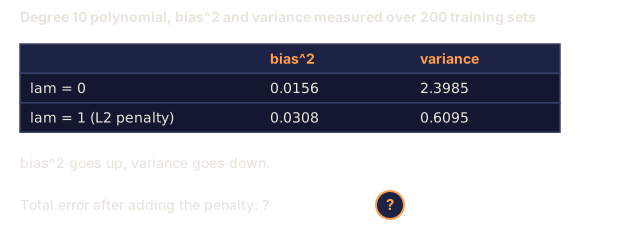
Regularization trades variance for bias on purpose: it constrains the model so it can't chase noise.
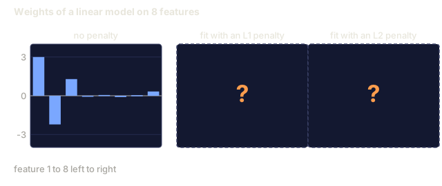
- L2 (Ridge): Shrinks all weights toward zero. Keeps all features but reduces their influence.
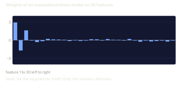
- L1 (Lasso): Pushes some weights exactly to zero. Performs feature selection.
- Dropout: Randomly disables neurons during training. Forces redundant representations.
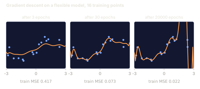
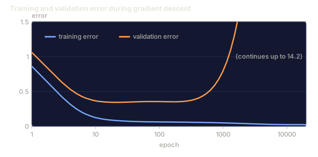
- Early stopping: Stops training before the model fully fits the training data.
The regularization strength (lambda, dropout rate, number of epochs) directly controls where you sit on the bias-variance curve. More regularization means more bias, less variance.
Double Descent: The Modern Perspective
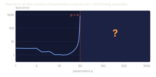
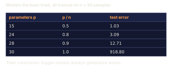
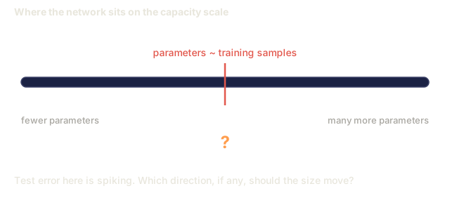
Classical theory says complexity past the sweet spot always hurts. Research since 2019 says otherwise: keep increasing model capacity far past the interpolation threshold, the point where the model has just enough parameters to fit the training data exactly, and test error can drop again.

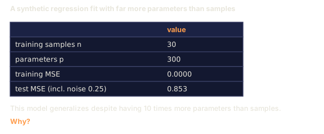
This "double descent" is why massively overparameterized neural networks, with far more parameters than training examples, still generalize. Classical bias-variance theory isn't wrong here, it's just incomplete once you're past the interpolation threshold.
Key observations about double descent:
- It shows up in linear models, decision trees, and neural networks alike
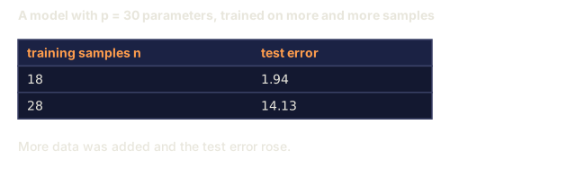
- More data can hurt in the interpolation region (sample-wise double descent)
- More training epochs can trigger it too (epoch-wise double descent)
- Regularization softens the peak but doesn't remove it
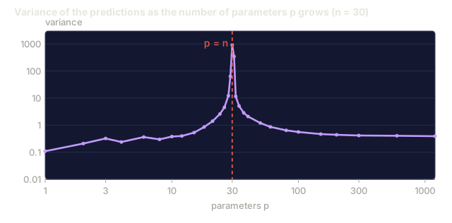
Why does this happen? At the interpolation threshold, the model has exactly enough capacity to fit every training point, so it gets forced into one very specific solution. Small perturbations in the data swing that solution wildly, which is why variance peaks right there. Past the threshold, many different solutions fit the data perfectly, and the learning algorithm (gradient descent with its implicit regularization, for instance) tends to land on the simplest one. That implicit bias toward simple solutions is the actual reason overparameterized models generalize.
| Regime | Parameters vs Samples | Behavior |
|---|---|---|
| Underparameterized | p << n | Classical tradeoff applies |
| Interpolation threshold | p ~ n | Variance peaks, test error spikes |
| Overparameterized | p >> n | Implicit regularization kicks in, test error drops |
Practical takeaway: if you're running neural networks or large tree ensembles, don't park at the interpolation threshold. Stay well below it with explicit regularization, or push well past it. The worst place to sit is right at the threshold.
Diagnosing Your Model

| Symptom | Diagnosis | Fix |
|---|---|---|
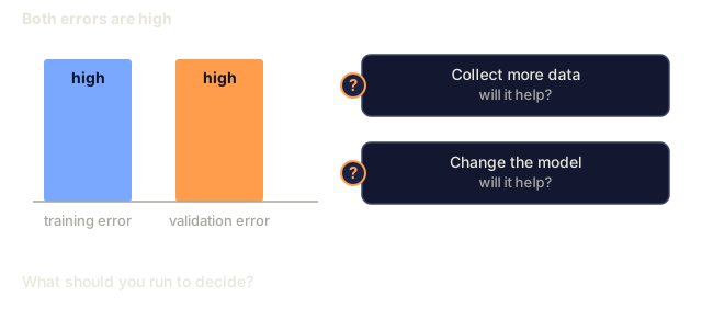
| High train error, high test error | Bias | More features, complex model, less regularization |
| Low train error, high test error | Variance | More data, regularization, simpler model, dropout |
| Low train error, low test error | Good fit | Ship it |
| Train error decreasing, test error increasing | Overfitting in progress | Early stopping |
Practical Strategies
When bias is the problem:
- Add polynomial or interaction features
- Use a more flexible model (tree ensemble instead of linear)
- Reduce regularization strength
- Train longer (if not yet converged)
When variance is the problem:
- Get more training data
- Use bagging (random forests)
- Increase regularization (higher lambda, more dropout)
- Feature selection (remove noisy features)
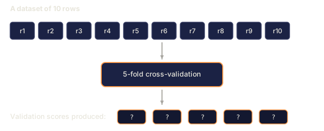
- Use cross-validation to detect it early
Ensemble Methods and Variance Reduction
Ensemble methods are the most practical tool you have for fighting variance.
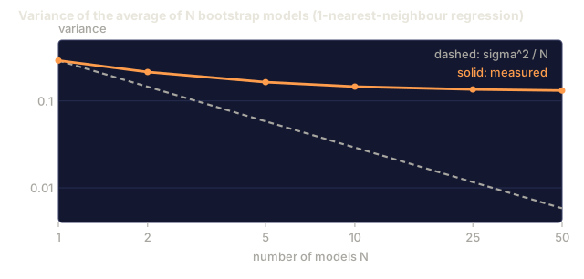
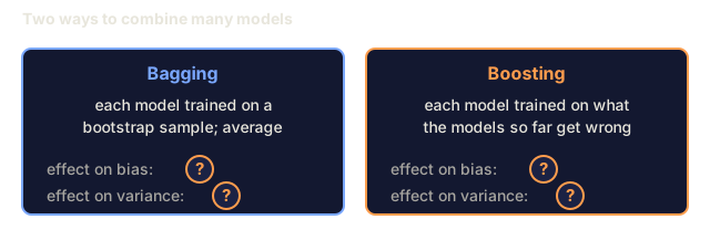
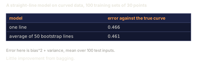
Bagging (Bootstrap Aggregating) draws many bootstrap samples (random resamples of the training data, drawn with replacement so the same row can appear more than once), trains one model per sample, then averages their predictions. Each individual model still has high variance, but averaging brings that variance down sharply. Random forests are bagging applied to decision trees.
Why it works mathematically: average N independent predictions, each with variance sigma^2, and the variance of the average drops to sigma^2 / N. The models aren't truly independent since they all see similar data, so the reduction falls short of 1/N. Still, it's substantial.
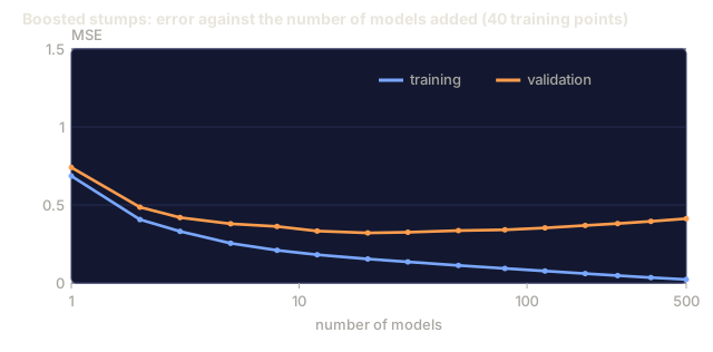
Boosting reduces bias by building models sequentially: each new model targets the errors the ensemble has made so far. Gradient boosting and AdaBoost are the main examples. Add too many models and boosting overfits, so you need early stopping or regularization to rein it in.
| Method | Primary Effect | Bias Change | Variance Change |
|---|---|---|---|
| Bagging | Reduces variance | No change | Decreases |
| Boosting | Reduces bias | Decreases | Can increase |
| Stacking | Reduces both | Depends on meta-learner | Depends on base models |
| Dropout | Implicit bagging | Slight increase | Decreases |
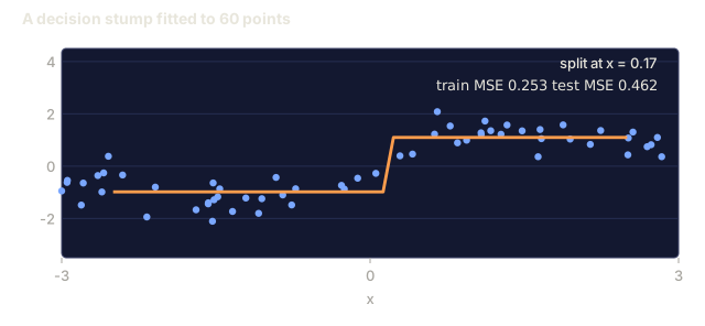
Practical rule: if your base model has high variance (deep trees, high-degree polynomials), use bagging. If it has high bias (shallow stumps, simple linear models), use boosting.
Learning Curves
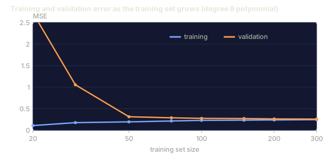
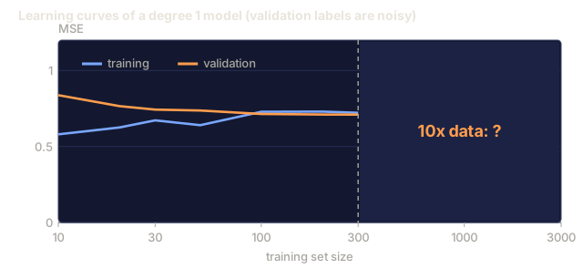
Learning curves plot training and validation error against training set size. They're the most practical diagnostic tool you have: unlike a single train/test comparison, they show you the model's trajectory and tell you whether more data will actually help.

How to read them:
| Scenario | Training Error | Validation Error | Gap | What It Means | What to Do |
|---|---|---|---|---|---|
| High bias | High | High | Small | Model cannot capture the pattern | More features, complex model, less regularization |
| High variance | Low | High | Large | Model memorizes training data | More data, regularization, simpler model |
| Good fit | Moderate | Moderate | Small | Model generalizes well | Ship it |
| High variance, improving | Low | Decreasing with more data | Shrinking | Variance problem that data can fix | Collect more data |
| High bias, flat | High | High and flat | Small and flat | More data will NOT help | Change model architecture |
The critical read: if both curves have flattened out with a small gap but both errors are still high, more data won't help. You need a better model. If the gap is large and still shrinking, more data will.
How to Generate Learning Curves
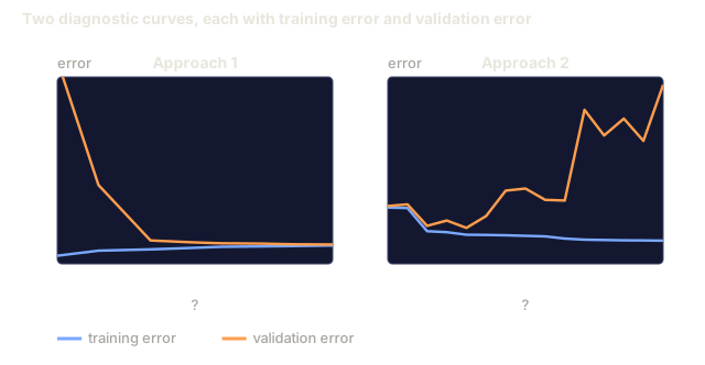
There are two approaches.
Approach 1: vary training set size, fixed model. Hold the model and hyperparameters constant, train on increasingly large subsets of the data, and measure training and validation error at each size. This is the standard learning curve.
Approach 2: vary model complexity, fixed data. Hold the data constant, sweep a complexity parameter (polynomial degree, tree depth, number of layers), and measure training and validation error at each setting. This is a validation curve, and it shows the bias-variance tradeoff directly.
The two complement each other: the first tells you if more data will help, the second tells you if a different model will help. Run both before deciding your next move.

Build It
code/bias_variance.py runs the full bias-variance decomposition experiment end to end. Here's the approach, step by step.
Step 1: Generate Synthetic Data from a Known Function
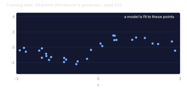
We use f(x) = sin(1.5x) + 0.5x with Gaussian noise on top. Knowing the true function up front is what lets us compute exact bias and variance instead of estimating them.
def true_function(x):
    return np.sin(1.5 * x) + 0.5 * x

def generate_data(n_samples=30, noise_std=0.5, x_range=(-3, 3), seed=None):
    rng = np.random.RandomState(seed)
    x = rng.uniform(x_range[0], x_range[1], n_samples)
    y = true_function(x) + rng.normal(0, noise_std, n_samples)
    return x, y
Step 2: Bootstrap Sampling and Polynomial Fitting
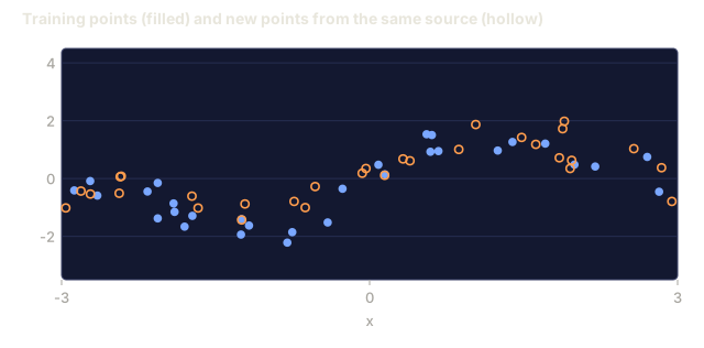
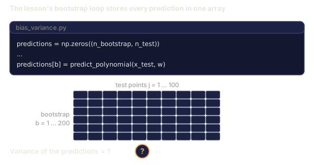
For each polynomial degree, we draw many bootstrap training sets, fit the polynomial, and record predictions on a fixed test grid. This gives us a distribution of predictions at each test point.
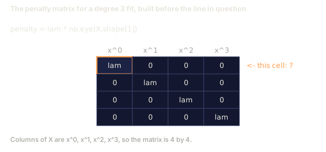
def fit_polynomial(x_train, y_train, degree, lam=0.0):
    X = np.column_stack([x_train ** d for d in range(degree + 1)])
    if lam > 0:
        penalty = lam * np.eye(X.shape[1])
        penalty[0, 0] = 0
        w = np.linalg.solve(X.T @ X + penalty, X.T @ y_train)
    else:
        w = np.linalg.lstsq(X, y_train, rcond=None)[0]
    return w
We fit this way across 200 different bootstrap samples, each drawn from the same underlying distribution but landing on different points.
Step 3: Computing Bias^2, Variance Decomposition
With 200 sets of predictions at each test point, we can compute the decomposition directly from the definition:
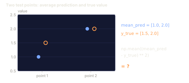
mean_pred = predictions.mean(axis=0)
bias_sq = np.mean((mean_pred - y_true) ** 2)
variance = np.mean(predictions.var(axis=0))
total_error = np.mean(np.mean((predictions - y_true) ** 2, axis=1))mean_predis E[f_hat(x)] estimated from bootstrap samplesbias_sqis the squared gap between average prediction and truthvarianceis the average spread of predictions across bootstrap samplestotal_errorshould approximately equal bias^2 + variance + noise
Step 4: Learning Curves
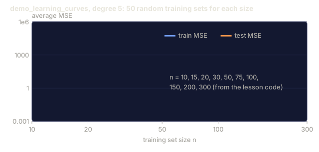
Learning curves sweep training set size while holding model complexity fixed. They show whether your model is data-limited or capacity-limited.
def demo_learning_curves():
    sizes = [10, 15, 20, 30, 50, 75, 100, 150, 200, 300]
    degree = 5

    for n in sizes:
        train_errors = []
        test_errors = []
        for seed in range(50):
            x_train, y_train = generate_data(n_samples=n, seed=seed * 100)
            w = fit_polynomial(x_train, y_train, degree)
            train_pred = predict_polynomial(x_train, w)
            train_mse = np.mean((train_pred - y_train) ** 2)
            test_pred = predict_polynomial(x_test, w)
            test_mse = np.mean((test_pred - y_test) ** 2)
            train_errors.append(train_mse)
            test_errors.append(test_mse)
        # Average over runs gives the learning curve point
For a high-variance model (degree 5 with small data), you see:
- Training error starts low and increases as more data makes memorization harder
- Test error starts high and decreases as the model gets more signal
- The gap shrinks with more data
For a high-bias model (degree 1), both errors converge quickly to the same high value and more data does not help.
Step 5: Regularization Sweep
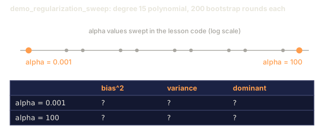
The code also includes demo_regularization_sweep(), which fixes a high-degree polynomial (degree 15) and sweeps Ridge strength from 0.001 to 100. It shows the same tradeoff from a different angle: instead of varying model complexity, we vary how hard the constraint bites.
def demo_regularization_sweep():
    alphas = [0.001, 0.005, 0.01, 0.05, 0.1, 0.5, 1.0, 5.0, 10.0, 50.0, 100.0]
    for alpha in alphas:
        results = bias_variance_decomposition([15], lam=alpha)
        r = results[15]
        print(f"alpha={alpha:.3f}  bias={r['bias_sq']:.4f}  var={r['variance']:.4f}")
At low alpha, the degree-15 polynomial is almost unconstrained and variance dominates: the model chases noise in every bootstrap sample. At high alpha, the penalty is so strong the model collapses to a near-constant function and bias takes over. The optimal alpha sits somewhere between the two extremes.
It's the same U-curve you get from varying polynomial degree, just controlled by a continuous knob instead of a discrete one. In practice, regularization is the preferred lever because it gives you fine-grained control without touching the feature set.
Use It
sklearn's learning_curve and validation_curve automate these diagnostics so you don't have to hand-roll the bootstrap loops yourself.
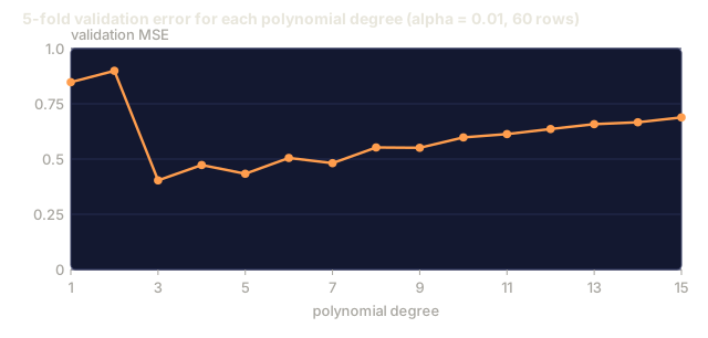
Validation Curve: Sweep Model Complexity
from sklearn.model_selection import validation_curve
from sklearn.pipeline import make_pipeline
from sklearn.preprocessing import PolynomialFeatures
from sklearn.linear_model import Ridge

degrees = list(range(1, 16))
train_scores_all = []
val_scores_all = []

for d in degrees:
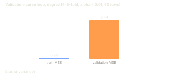
    pipe = make_pipeline(PolynomialFeatures(d), Ridge(alpha=0.01))
    train_scores, val_scores = validation_curve(
        pipe, X, y, param_name="polynomialfeatures__degree",
        param_range=[d], cv=5, scoring="neg_mean_squared_error"
    )
    train_scores_all.append(-train_scores.mean())
    val_scores_all.append(-val_scores.mean())
This traces the bias-variance tradeoff curve directly: wherever the validation score lags train score badly, variance dominates, and wherever both are bad, bias does.
Learning Curve: Sweep Training Set Size
from sklearn.model_selection import learning_curve

pipe = make_pipeline(PolynomialFeatures(5), Ridge(alpha=0.01))
train_sizes, train_scores, val_scores = learning_curve(
    pipe, X, y, train_sizes=np.linspace(0.1, 1.0, 10),
    cv=5, scoring="neg_mean_squared_error"
)
train_mse = -train_scores.mean(axis=1)
val_mse = -val_scores.mean(axis=1)
Plot train_mse and val_mse against train_sizes. The shape tells you everything about your model.
Cross-Validation with Regularization Sweep
from sklearn.model_selection import cross_val_score

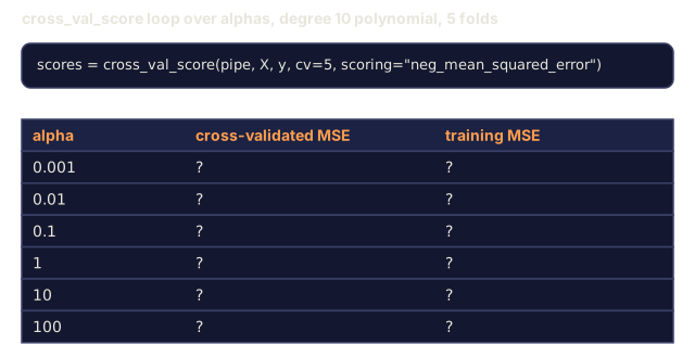
alphas = [0.001, 0.01, 0.1, 1.0, 10.0, 100.0]
for alpha in alphas:
    pipe = make_pipeline(PolynomialFeatures(10), Ridge(alpha=alpha))
    scores = cross_val_score(pipe, X, y, cv=5, scoring="neg_mean_squared_error")
    print(f"alpha={alpha:>7.3f}  MSE={-scores.mean():.4f} +/- {scores.std():.4f}")
This sweeps regularization strength for a fixed model complexity. You will see the same bias-variance tradeoff: low alpha means high variance, high alpha means high bias.
Putting It All Together: A Complete Diagnostic Workflow
In practice, you run these diagnostics in sequence:
- Train your model. Compute train and test error.
- If both are high: you have a bias problem. Skip to step 4.
- If train is low but test is high: you have a variance problem. Generate a learning curve to see if more data will help. If not, regularize.
- Generate a validation curve sweeping your main complexity parameter. Find the sweet spot.
- At the sweet spot, generate a learning curve. If the gap is still large, you need more data or regularization.
- Try Ridge/Lasso with different alpha values using
cross_val_score. Pick the alpha where cross-validated error is lowest.
This takes 10-15 minutes of compute for most tabular datasets and saves hours of guessing.
Ship It
This lesson produces: outputs/prompt-model-diagnostics.md
The double descent section is the one people file away as trivia and then get burned by later. If you're fitting a small linear model, the classical U-curve is the whole story and you can stop there. But the moment you're staring at a neural network with more parameters than training examples that's still generalizing fine, the classical story alone will make you second-guess a model that's actually working. Know which regime you're in before you start regularizing on instinct.
The other thing worth saying directly: bias and variance aren't properties of a model. They're properties of a model plus a dataset plus a training procedure. Change any one of those and a high-bias problem can turn into a high-variance one. Rerun the diagnosis every time something upstream changes. Don't coast on last month's conclusion.
Exercises
-
Run the decomposition with
noise_std=0(no noise). What happens to the irreducible error term? Does the optimal complexity change? -
Increase the training set size from 30 to 300. How does this affect the variance component? Does the optimal polynomial degree shift?
-
Add L2 regularization (Ridge regression) to the experiment. For a fixed high-degree polynomial (degree 15), sweep lambda from 0 to 100. Plot bias^2 and variance as functions of lambda.
-
Modify the true function from a polynomial to
sin(x). How does the bias-variance decomposition change? Is there still a clear optimal degree? -
Implement a simple bootstrap aggregating (bagging) wrapper: train 10 models on bootstrap samples and average predictions. Show that this reduces variance without increasing bias much.
Key Terms
| Term | What people say | What it actually means |
|---|---|---|
| Bias | "The model is too simple" | Systematic error from wrong assumptions. The gap between the average model prediction and truth. |
| Variance | "The model is overfitting" | Error from sensitivity to training data. How much predictions change across different training sets. |
| Irreducible error | "Noise in the data" | Error from randomness in the true data-generating process. No model can eliminate it. |
| Underfitting | "Not learning enough" | Model has high bias. It misses the real pattern even on training data. |
| Overfitting | "Memorizing the data" | Model has high variance. It fits noise in training data that does not generalize. |
| Regularization | "Constraining the model" | Adding a penalty to reduce model complexity, trading bias for lower variance. |
| Double descent | "More parameters can help" | Test error decreases again when model capacity far exceeds the interpolation threshold. |
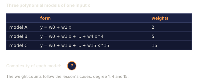
| Model complexity | "How flexible the model is" | The capacity of a model to fit arbitrary patterns. Controlled by architecture, features, or regularization. |
Further Reading
- Hastie, Tibshirani, Friedman: Elements of Statistical Learning, Ch. 7 -- the definitive treatment of bias-variance decomposition
- Belkin et al., Reconciling modern machine learning practice and the bias-variance trade-off (2019) -- the double descent paper
- Nakkiran et al., Deep Double Descent (2019) -- epoch-wise and sample-wise double descent
- Scott Fortmann-Roe: Understanding the Bias-Variance Tradeoff -- clear visual explanation
Code
- bias_variance.py (python, 325 lines)