Model Evaluation
A model is only as good as the way you measure it. Get the measurement wrong and every decision downstream of it, which model to ship, which feature to cut, is a guess dressed up as data.
Learning Objectives
- Implement K-fold and stratified K-fold cross-validation from scratch and explain why stratification matters for imbalanced data
- Compute precision, recall, F1, AUC-ROC, and regression metrics (MSE, RMSE, MAE, R-squared) from scratch
- Interpret learning curves to diagnose whether a model suffers from high bias or high variance
- Identify common evaluation mistakes including data leakage, wrong metric selection, and test set contamination
The Problem
You trained a model. It scores 95% accuracy. Good, right?
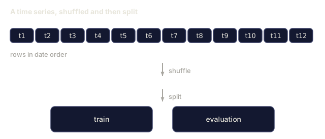
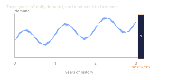
Not necessarily. If 95% of your labels belong to one class, a model that always predicts that class also scores 95%, and it's worthless. Evaluate on the same rows you trained on and that number stops meaning anything, because the model just memorized the answers instead of learning to generalize. Shuffle a time-series dataset before splitting and you can end up training on the future to predict the past without ever noticing.
This is where most ML projects actually fail: not at the modeling step, at the measurement step. The wrong metric makes a bad model look great. The wrong split lets a model cheat. The wrong comparison talks you into shipping the worse of two options. Get evaluation right and you know what you actually have. Get it wrong and you find out in production, which is the most expensive place to find out.

The Concept
Train, Validation, Test

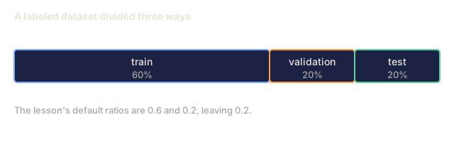
Three splits, three jobs:
- Training set: the model learns from this data, seeing every example during training.
- Validation set: used to tune hyperparameters and choose between models. The model never trains on it, but every decision you make is shaped by it.
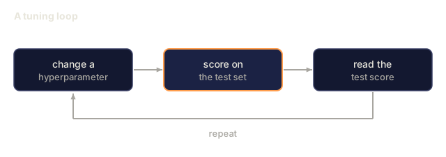
- Test set: touched exactly once, at the very end, to report final performance. Look at test performance, adjust the model, and look again, and it stops being a test set: it's just become a second validation set.
The test set is the one number in this whole process you can actually trust to describe how the model behaves on data it has never seen.
K-Fold Cross-Validation
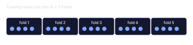
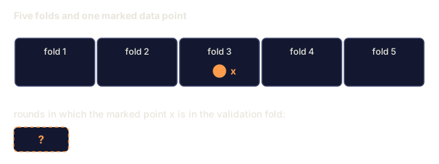
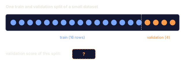
K-fold cross-validation splits the data into K folds, trains on K-1 of them, and validates on whichever fold is left out, rotating through all K until every point has served as both training and validation data. It exists to fix a real problem: with a small dataset, one single train/validation split wastes data you can't afford to waste and gives you a noisy read on true performance.

- Split data into K equal-sized folds
- For each fold, train on K-1 folds and validate on the remaining fold
- Average the K validation scores
K=5 or K=10 are the standard choices. Every data point gets used for validation exactly once, and the averaged score is a far more stable estimate than anything a single split can give you.
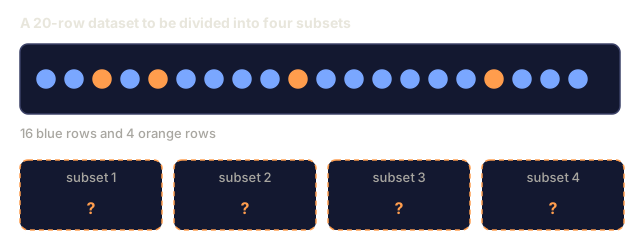
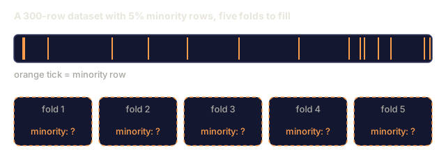
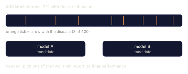
Stratified K-fold preserves the class ratio within every fold. A dataset that's 70% class A and 30% class B keeps roughly that same 70/30 split inside each fold. That matters most on imbalanced data, where an unlucky random split could otherwise dump nearly all the minority-class rows into one fold.
Classification Metrics
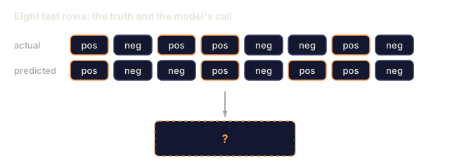
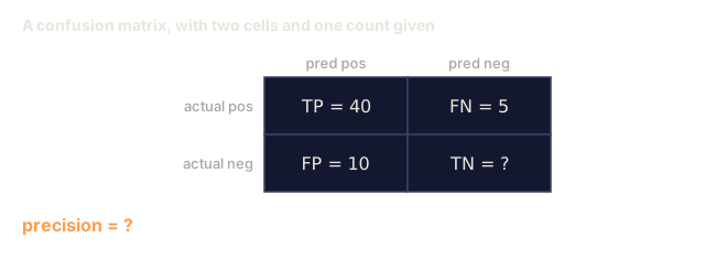
Confusion matrix: the table everything else in this section gets computed from. For binary classification:
| Predicted Positive | Predicted Negative | |
|---|---|---|
| Actually Positive | True Positive (TP) | False Negative (FN) |
| Actually Negative | False Positive (FP) | True Negative (TN) |
Every other metric here is just arithmetic on these four counts:
- Accuracy = (TP + TN) / (TP + TN + FP + FN). The fraction of predictions that were correct. Misleading the moment your classes are imbalanced.
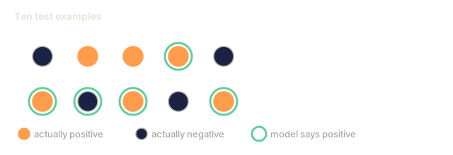
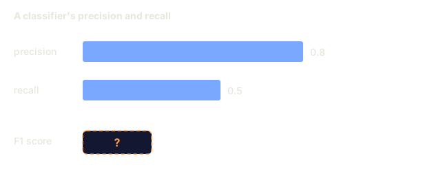
- Precision = TP / (TP + FP). Of everything you predicted positive, how much actually was? Use this when false positives are the expensive mistake, like a spam filter burying a real email.
- Recall (sensitivity) = TP / (TP + FN). Of everything that was actually positive, how much did you catch? Use this when false negatives are the expensive mistake, like a cancer screening missing a tumor.
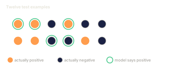
- F1 score = 2 * precision * recall / (precision + recall). The harmonic mean of precision and recall, for when neither one clearly matters more than the other.
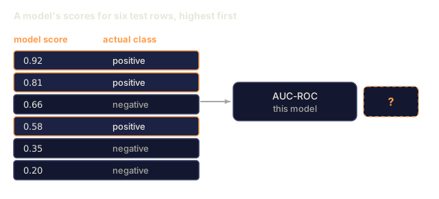
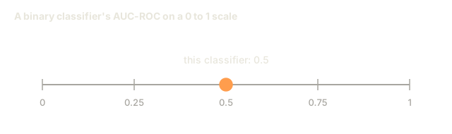
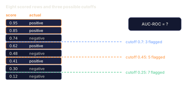
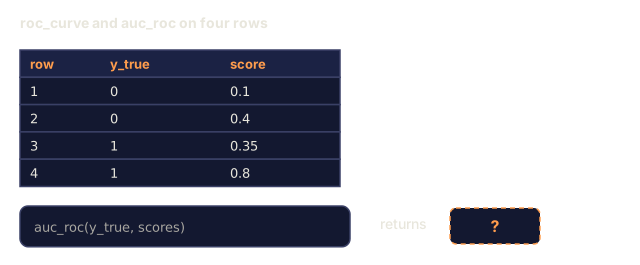
- AUC-ROC: the area under the Receiver Operating Characteristic curve, which plots true positive rate against false positive rate across every possible classification threshold. AUC = 0.5 is random guessing, AUC = 1.0 is perfect separation. It's threshold-independent: it measures how well the model ranks positives above negatives, no matter which cutoff you eventually pick.
Regression Metrics
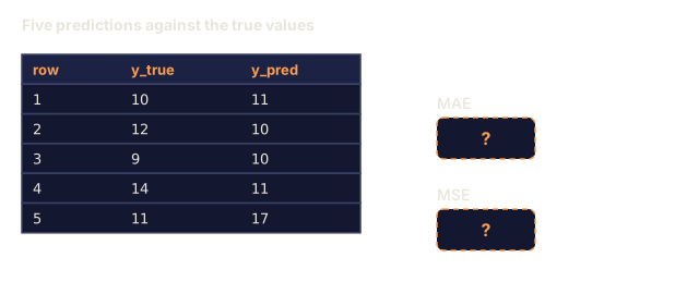
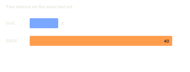
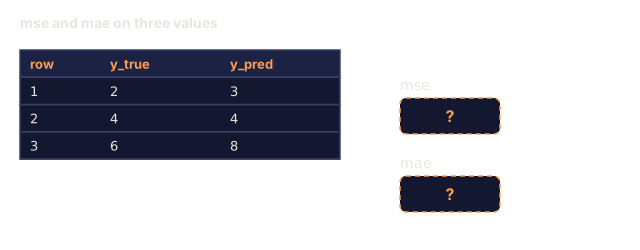
- MSE (Mean Squared Error) = mean((y_true - y_pred)^2). Penalizes large errors quadratically, so it's sensitive to outliers.
- RMSE (Root Mean Squared Error) = sqrt(MSE). Same units as the target variable, which makes it easier to interpret than MSE.
- MAE (Mean Absolute Error) = mean(|y_true - y_pred|). Treats every error linearly, which makes it less sensitive to outliers than MSE.
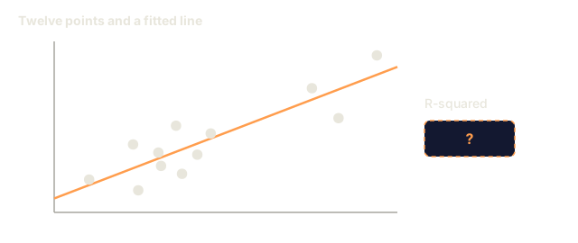
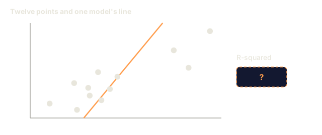
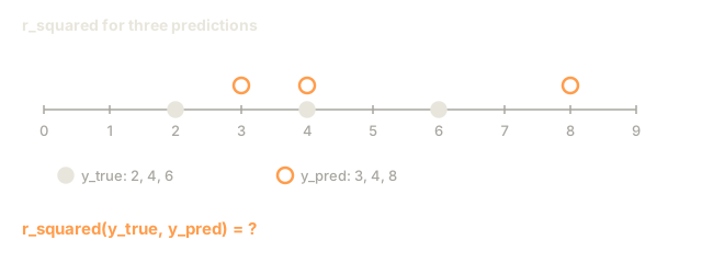
- R-squared = 1 - SS_res / SS_tot, where SS_res = sum((y_true - y_pred)^2) and SS_tot = sum((y_true - y_mean)^2). The fraction of variance the model explains. R^2 = 1.0 is perfect, R^2 = 0.0 means the model is no better than always predicting the mean, and R^2 can go negative if the model is worse than that.
Learning Curves
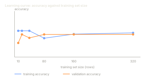
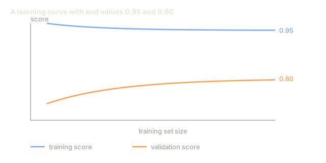
A learning curve plots training and validation scores against training set size:
- High bias (underfitting): both curves converge to a low score. More data won't help here; what you need is a more complex model.
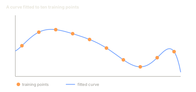
- High variance (overfitting): training score is high, validation score is much lower, and the gap between them is wide. More data should close that gap.
Validation Curves
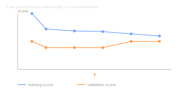
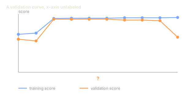
A validation curve plots the same two scores, but against a hyperparameter instead of training set size:
- At low complexity: both scores are low (underfitting)
- At the right complexity: both scores are high and close together
- At high complexity: training score stays high but validation score drops (overfitting)
The best hyperparameter value sits wherever the validation score peaks.
Common Evaluation Mistakes
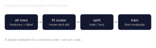
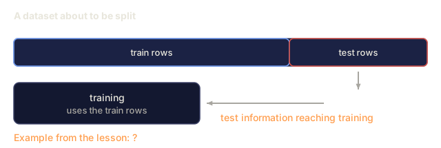
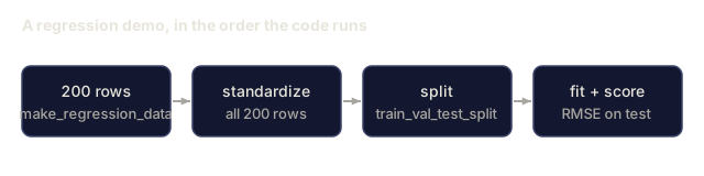
Data leakage: information from the test set leaks into training. It shows up as fitting a scaler on the full dataset before splitting, letting future data slip into a time series prediction, or using a feature that's secretly derived from the target. The fix is always the same order of operations: split first, then preprocess.
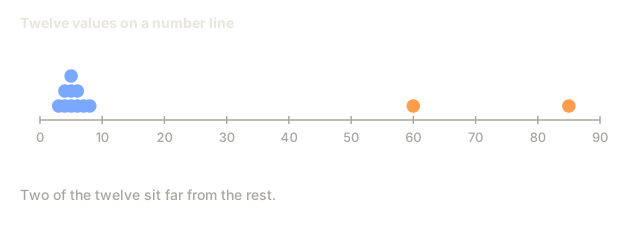
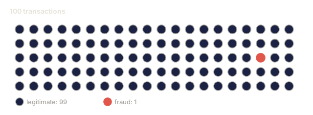
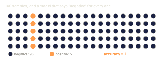
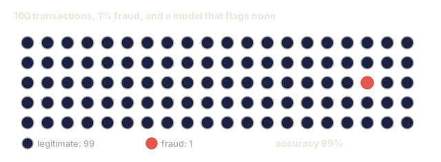
Class imbalance: 99% of transactions are legitimate, 1% are fraud. A model that predicts "legitimate" every single time still gets 99% accuracy. Use precision, recall, F1, or AUC-ROC instead, because accuracy can't tell you this model is useless.
Wrong metric: optimizing accuracy when you should be optimizing recall, as in medical diagnosis, or optimizing RMSE when your data is full of outliers, when MAE would serve you better.
Not using stratified splits: on imbalanced data, a plain random split can leave the validation fold with almost no minority samples, and your estimate becomes unstable.
Testing too often: every time you check test performance and adjust the model in response, you overfit to the test set a little more. It's single-use for a reason.


Build It
Step 1: Train/validation/test split
import random
import math


def train_val_test_split(X, y, train_ratio=0.6, val_ratio=0.2, seed=42):
    random.seed(seed)
    n = len(X)
    indices = list(range(n))
    random.shuffle(indices)

    train_end = int(n * train_ratio)
    val_end = int(n * (train_ratio + val_ratio))

    train_idx = indices[:train_end]
    val_idx = indices[train_end:val_end]
    test_idx = indices[val_end:]

    X_train = [X[i] for i in train_idx]
    y_train = [y[i] for i in train_idx]
    X_val = [X[i] for i in val_idx]
    y_val = [y[i] for i in val_idx]
    X_test = [X[i] for i in test_idx]
    y_test = [y[i] for i in test_idx]

    return X_train, y_train, X_val, y_val, X_test, y_test
Step 2: K-fold and stratified K-fold cross-validation
def kfold_split(n, k=5, seed=42):
    random.seed(seed)
    indices = list(range(n))
    random.shuffle(indices)

    fold_size = n // k
    folds = []

    for i in range(k):
        start = i * fold_size
        end = start + fold_size if i < k - 1 else n
        val_idx = indices[start:end]
        train_idx = indices[:start] + indices[end:]
        folds.append((train_idx, val_idx))

    return folds


def stratified_kfold_split(y, k=5, seed=42):
    random.seed(seed)

    class_indices = {}
    for i, label in enumerate(y):
        class_indices.setdefault(label, []).append(i)

    for label in class_indices:
        random.shuffle(class_indices[label])

    folds = [{"train": [], "val": []} for _ in range(k)]

    for label, indices in class_indices.items():
        fold_size = len(indices) // k
        for i in range(k):
            start = i * fold_size
            end = start + fold_size if i < k - 1 else len(indices)
            val_part = indices[start:end]
            train_part = indices[:start] + indices[end:]
            folds[i]["val"].extend(val_part)
            folds[i]["train"].extend(train_part)

    return [(f["train"], f["val"]) for f in folds]


def cross_validate(X, y, model_fn, k=5, metric_fn=None, stratified=False):
    n = len(X)

    if stratified:
        folds = stratified_kfold_split(y, k)
    else:
        folds = kfold_split(n, k)

    scores = []
    for train_idx, val_idx in folds:
        X_train = [X[i] for i in train_idx]
        y_train = [y[i] for i in train_idx]
        X_val = [X[i] for i in val_idx]
        y_val = [y[i] for i in val_idx]

        model = model_fn()
        model.fit(X_train, y_train)
        predictions = [model.predict(x) for x in X_val]

        if metric_fn:
            score = metric_fn(y_val, predictions)
        else:
            score = sum(1 for yt, yp in zip(y_val, predictions) if yt == yp) / len(y_val)
        scores.append(score)

    return scores
Step 3: Confusion matrix and classification metrics
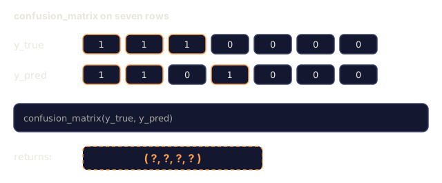
def confusion_matrix(y_true, y_pred):
    tp = sum(1 for yt, yp in zip(y_true, y_pred) if yt == 1 and yp == 1)
    tn = sum(1 for yt, yp in zip(y_true, y_pred) if yt == 0 and yp == 0)
    fp = sum(1 for yt, yp in zip(y_true, y_pred) if yt == 0 and yp == 1)
    fn = sum(1 for yt, yp in zip(y_true, y_pred) if yt == 1 and yp == 0)
    return tp, tn, fp, fn


def accuracy(y_true, y_pred):
    tp, tn, fp, fn = confusion_matrix(y_true, y_pred)
    total = tp + tn + fp + fn
    return (tp + tn) / total if total > 0 else 0.0


def precision(y_true, y_pred):
    tp, tn, fp, fn = confusion_matrix(y_true, y_pred)
    return tp / (tp + fp) if (tp + fp) > 0 else 0.0


def recall(y_true, y_pred):
    tp, tn, fp, fn = confusion_matrix(y_true, y_pred)
    return tp / (tp + fn) if (tp + fn) > 0 else 0.0


def f1_score(y_true, y_pred):
    p = precision(y_true, y_pred)
    r = recall(y_true, y_pred)
    return 2 * p * r / (p + r) if (p + r) > 0 else 0.0


def roc_curve(y_true, y_scores):
    thresholds = sorted(set(y_scores), reverse=True)
    tpr_list = []
    fpr_list = []

    total_positives = sum(y_true)
    total_negatives = len(y_true) - total_positives

    for threshold in thresholds:
        y_pred = [1 if s >= threshold else 0 for s in y_scores]
        tp = sum(1 for yt, yp in zip(y_true, y_pred) if yt == 1 and yp == 1)
        fp = sum(1 for yt, yp in zip(y_true, y_pred) if yt == 0 and yp == 1)

        tpr = tp / total_positives if total_positives > 0 else 0.0
        fpr = fp / total_negatives if total_negatives > 0 else 0.0

        tpr_list.append(tpr)
        fpr_list.append(fpr)

    return fpr_list, tpr_list, thresholds


def auc_roc(y_true, y_scores):
    fpr_list, tpr_list, _ = roc_curve(y_true, y_scores)

    pairs = sorted(zip(fpr_list, tpr_list))
    fpr_sorted = [p[0] for p in pairs]
    tpr_sorted = [p[1] for p in pairs]

    area = 0.0
    for i in range(1, len(fpr_sorted)):
        width = fpr_sorted[i] - fpr_sorted[i - 1]
        height = (tpr_sorted[i] + tpr_sorted[i - 1]) / 2
        area += width * height

    return area
Step 4: Regression metrics
def mse(y_true, y_pred):
    n = len(y_true)
    return sum((yt - yp) ** 2 for yt, yp in zip(y_true, y_pred)) / n


def rmse(y_true, y_pred):
    return math.sqrt(mse(y_true, y_pred))


def mae(y_true, y_pred):
    n = len(y_true)
    return sum(abs(yt - yp) for yt, yp in zip(y_true, y_pred)) / n


def r_squared(y_true, y_pred):
    mean_y = sum(y_true) / len(y_true)
    ss_res = sum((yt - yp) ** 2 for yt, yp in zip(y_true, y_pred))
    ss_tot = sum((yt - mean_y) ** 2 for yt in y_true)
    if ss_tot == 0:
        return 0.0
    return 1.0 - ss_res / ss_tot
Step 5: Learning curves
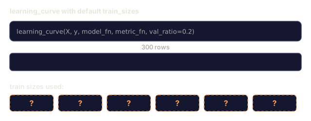
def learning_curve(X, y, model_fn, metric_fn, train_sizes=None, val_ratio=0.2, seed=42):
    random.seed(seed)
    n = len(X)
    indices = list(range(n))
    random.shuffle(indices)

    val_size = int(n * val_ratio)
    val_idx = indices[:val_size]
    pool_idx = indices[val_size:]

    X_val = [X[i] for i in val_idx]
    y_val = [y[i] for i in val_idx]

    if train_sizes is None:
        train_sizes = [int(len(pool_idx) * r) for r in [0.1, 0.2, 0.4, 0.6, 0.8, 1.0]]

    train_scores = []
    val_scores = []

    for size in train_sizes:
        subset = pool_idx[:size]
        X_train = [X[i] for i in subset]
        y_train = [y[i] for i in subset]

        model = model_fn()
        model.fit(X_train, y_train)

        train_pred = [model.predict(x) for x in X_train]
        val_pred = [model.predict(x) for x in X_val]

        train_scores.append(metric_fn(y_train, train_pred))
        val_scores.append(metric_fn(y_val, val_pred))

    return train_sizes, train_scores, val_scores
Step 6: A simple classifier for testing, plus the full demo
class SimpleLogistic:
    def __init__(self, lr=0.1, epochs=100):
        self.lr = lr
        self.epochs = epochs
        self.weights = None
        self.bias = 0.0

    def sigmoid(self, z):
        z = max(-500, min(500, z))
        return 1.0 / (1.0 + math.exp(-z))

    def fit(self, X, y):
        n_features = len(X[0])
        self.weights = [0.0] * n_features
        self.bias = 0.0

        for _ in range(self.epochs):
            for xi, yi in zip(X, y):
                z = sum(w * x for w, x in zip(self.weights, xi)) + self.bias
                pred = self.sigmoid(z)
                error = yi - pred
                for j in range(n_features):
                    self.weights[j] += self.lr * error * xi[j]
                self.bias += self.lr * error

    def predict_proba(self, x):
        z = sum(w * xi for w, xi in zip(self.weights, x)) + self.bias
        return self.sigmoid(z)

    def predict(self, x):
        return 1 if self.predict_proba(x) >= 0.5 else 0


class SimpleLinearRegression:
    def __init__(self, lr=0.001, epochs=200):
        self.lr = lr
        self.epochs = epochs
        self.weights = None
        self.bias = 0.0

    def fit(self, X, y):
        n_features = len(X[0])
        self.weights = [0.0] * n_features
        self.bias = 0.0
        n = len(X)

        for _ in range(self.epochs):
            for xi, yi in zip(X, y):
                pred = sum(w * x for w, x in zip(self.weights, xi)) + self.bias
                error = yi - pred
                for j in range(n_features):
                    self.weights[j] += self.lr * error * xi[j] / n
                self.bias += self.lr * error / n

    def predict(self, x):
        return sum(w * xi for w, xi in zip(self.weights, x)) + self.bias


def standardize(values):
    n = len(values)
    mean = sum(values) / n
    var = sum((v - mean) ** 2 for v in values) / n
    std = math.sqrt(var) if var > 0 else 1.0
    return [(v - mean) / std for v in values], mean, std


def make_classification_data(n=300, seed=42):
    random.seed(seed)
    X = []
    y = []
    for _ in range(n):
        x1 = random.gauss(0, 1)
        x2 = random.gauss(0, 1)
        label = 1 if (x1 + x2 + random.gauss(0, 0.5)) > 0 else 0
        X.append([x1, x2])
        y.append(label)
    return X, y


def make_regression_data(n=200, seed=42):
    random.seed(seed)
    X = []
    y = []
    for _ in range(n):
        x1 = random.uniform(0, 10)
        x2 = random.uniform(0, 5)
        target = 3 * x1 + 2 * x2 + random.gauss(0, 2)
        X.append([x1, x2])
        y.append(target)
    return X, y


def make_imbalanced_data(n=300, minority_ratio=0.05, seed=42):
    random.seed(seed)
    X = []
    y = []
    for _ in range(n):
        if random.random() < minority_ratio:
            x1 = random.gauss(3, 0.5)
            x2 = random.gauss(3, 0.5)
            label = 1
        else:
            x1 = random.gauss(0, 1)
            x2 = random.gauss(0, 1)
            label = 0
        X.append([x1, x2])
        y.append(label)
    return X, y


if __name__ == "__main__":
    X_clf, y_clf = make_classification_data(300)

    print("=== Train/Validation/Test Split ===")
    X_train, y_train, X_val, y_val, X_test, y_test = train_val_test_split(X_clf, y_clf)
    print(f"  Train: {len(X_train)}, Val: {len(X_val)}, Test: {len(X_test)}")
    print(f"  Train class distribution: {sum(y_train)}/{len(y_train)} positive")
    print(f"  Val class distribution: {sum(y_val)}/{len(y_val)} positive")

    model = SimpleLogistic(lr=0.1, epochs=200)
    model.fit(X_train, y_train)

    print("\n=== Classification Metrics ===")
    y_pred = [model.predict(x) for x in X_test]
    tp, tn, fp, fn = confusion_matrix(y_test, y_pred)
    print(f"  Confusion matrix: TP={tp}, TN={tn}, FP={fp}, FN={fn}")
    print(f"  Accuracy:  {accuracy(y_test, y_pred):.4f}")
    print(f"  Precision: {precision(y_test, y_pred):.4f}")
    print(f"  Recall:    {recall(y_test, y_pred):.4f}")
    print(f"  F1 Score:  {f1_score(y_test, y_pred):.4f}")

    y_scores = [model.predict_proba(x) for x in X_test]
    auc = auc_roc(y_test, y_scores)
    print(f"  AUC-ROC:   {auc:.4f}")

    print("\n=== K-Fold Cross-Validation (K=5) ===")
    cv_scores = cross_validate(
        X_clf, y_clf,
        model_fn=lambda: SimpleLogistic(lr=0.1, epochs=200),
        k=5,
        metric_fn=accuracy,
    )
    mean_cv = sum(cv_scores) / len(cv_scores)
    std_cv = math.sqrt(sum((s - mean_cv) ** 2 for s in cv_scores) / len(cv_scores))
    print(f"  Fold scores: {[round(s, 4) for s in cv_scores]}")
    print(f"  Mean: {mean_cv:.4f} (+/- {std_cv:.4f})")

    print("\n=== Stratified K-Fold Cross-Validation (K=5) ===")
    strat_scores = cross_validate(
        X_clf, y_clf,
        model_fn=lambda: SimpleLogistic(lr=0.1, epochs=200),
        k=5,
        metric_fn=accuracy,
        stratified=True,
    )
    strat_mean = sum(strat_scores) / len(strat_scores)
    strat_std = math.sqrt(sum((s - strat_mean) ** 2 for s in strat_scores) / len(strat_scores))
    print(f"  Fold scores: {[round(s, 4) for s in strat_scores]}")
    print(f"  Mean: {strat_mean:.4f} (+/- {strat_std:.4f})")

    print("\n=== Imbalanced Data: Why Accuracy Lies ===")
    X_imb, y_imb = make_imbalanced_data(300, minority_ratio=0.05)
    positives = sum(y_imb)
    print(f"  Class distribution: {positives} positive, {len(y_imb) - positives} negative ({positives/len(y_imb)*100:.1f}% positive)")

    always_negative = [0] * len(y_imb)
    print(f"  Always-negative baseline:")
    print(f"    Accuracy:  {accuracy(y_imb, always_negative):.4f}")
    print(f"    Precision: {precision(y_imb, always_negative):.4f}")
    print(f"    Recall:    {recall(y_imb, always_negative):.4f}")
    print(f"    F1 Score:  {f1_score(y_imb, always_negative):.4f}")

    X_tr_i, y_tr_i, X_v_i, y_v_i, X_te_i, y_te_i = train_val_test_split(X_imb, y_imb)
    model_imb = SimpleLogistic(lr=0.5, epochs=500)
    model_imb.fit(X_tr_i, y_tr_i)
    y_pred_imb = [model_imb.predict(x) for x in X_te_i]
    print(f"\n  Trained model on imbalanced data:")
    print(f"    Accuracy:  {accuracy(y_te_i, y_pred_imb):.4f}")
    print(f"    Precision: {precision(y_te_i, y_pred_imb):.4f}")
    print(f"    Recall:    {recall(y_te_i, y_pred_imb):.4f}")
    print(f"    F1 Score:  {f1_score(y_te_i, y_pred_imb):.4f}")

    print("\n=== Regression Metrics ===")
    X_reg, y_reg = make_regression_data(200)

    col0 = [x[0] for x in X_reg]
    col1 = [x[1] for x in X_reg]
    col0_s, m0, s0 = standardize(col0)
    col1_s, m1, s1 = standardize(col1)
    X_reg_scaled = [[col0_s[i], col1_s[i]] for i in range(len(X_reg))]

    X_tr_r, y_tr_r, X_v_r, y_v_r, X_te_r, y_te_r = train_val_test_split(X_reg_scaled, y_reg)
    reg_model = SimpleLinearRegression(lr=0.01, epochs=500)
    reg_model.fit(X_tr_r, y_tr_r)
    y_pred_r = [reg_model.predict(x) for x in X_te_r]

    print(f"  MSE:       {mse(y_te_r, y_pred_r):.4f}")
    print(f"  RMSE:      {rmse(y_te_r, y_pred_r):.4f}")
    print(f"  MAE:       {mae(y_te_r, y_pred_r):.4f}")
    print(f"  R-squared: {r_squared(y_te_r, y_pred_r):.4f}")

    mean_baseline = [sum(y_tr_r) / len(y_tr_r)] * len(y_te_r)
    print(f"\n  Mean baseline:")
    print(f"    MSE:       {mse(y_te_r, mean_baseline):.4f}")
    print(f"    R-squared: {r_squared(y_te_r, mean_baseline):.4f}")

    print("\n=== Learning Curve ===")
    sizes, train_sc, val_sc = learning_curve(
        X_clf, y_clf,
        model_fn=lambda: SimpleLogistic(lr=0.1, epochs=200),
        metric_fn=accuracy,
    )
    print(f"  {'Size':>6} {'Train':>8} {'Val':>8}")
    for s, tr, va in zip(sizes, train_sc, val_sc):
        print(f"  {s:>6} {tr:>8.4f} {va:>8.4f}")

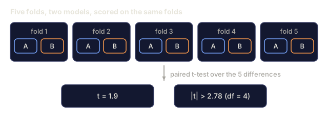
    print("\n=== Statistical Model Comparison ===")
    model_a_scores = cross_validate(
        X_clf, y_clf,
        model_fn=lambda: SimpleLogistic(lr=0.1, epochs=100),
        k=5, metric_fn=accuracy,
    )
    model_b_scores = cross_validate(
        X_clf, y_clf,
        model_fn=lambda: SimpleLogistic(lr=0.1, epochs=500),
        k=5, metric_fn=accuracy,
    )
    diffs = [a - b for a, b in zip(model_a_scores, model_b_scores)]
    mean_diff = sum(diffs) / len(diffs)
    std_diff = math.sqrt(sum((d - mean_diff) ** 2 for d in diffs) / len(diffs))
    t_stat = mean_diff / (std_diff / math.sqrt(len(diffs))) if std_diff > 0 else 0.0
    print(f"  Model A (100 epochs) mean: {sum(model_a_scores)/len(model_a_scores):.4f}")
    print(f"  Model B (500 epochs) mean: {sum(model_b_scores)/len(model_b_scores):.4f}")
    print(f"  Mean difference: {mean_diff:.4f}")
    print(f"  Paired t-statistic: {t_stat:.4f}")
    print(f"  (|t| > 2.78 for significance at p<0.05 with df=4)")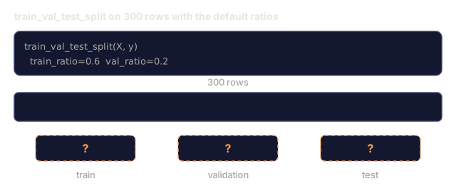
Use It
With scikit-learn, all of this evaluation machinery is already wired into the workflow:
from sklearn.model_selection import cross_val_score, StratifiedKFold, learning_curve
from sklearn.metrics import (
    accuracy_score, precision_score, recall_score, f1_score,
    roc_auc_score, confusion_matrix, mean_squared_error, r2_score,
)
from sklearn.linear_model import LogisticRegression

model = LogisticRegression()
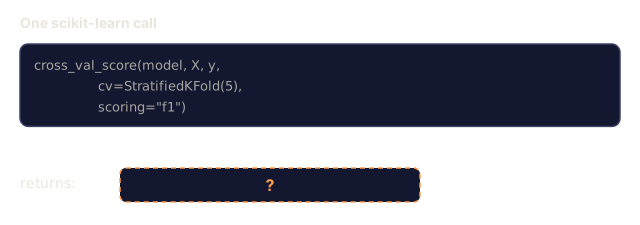
scores = cross_val_score(model, X, y, cv=StratifiedKFold(5), scoring="f1")
The from-scratch code above wasn't wasted effort. It shows exactly what cross-validation does under the hood (for-loops and index tracking, no magic), how each metric reduces to counting TP/FP/TN/FN, and why stratification matters (it preserves the class ratio inside every fold). Scikit-learn's versions add what you actually want once you're past learning it: parallelism, more scoring options, and pipeline integration.
Ship It
This lesson ships:
outputs/skill-evaluation.md: a skill covering evaluation strategy for classification and regression models
The mistake that costs people the most in practice isn't picking the wrong metric. It's peeking. You run cross-validation, look at the fold scores, tweak a hyperparameter because fold 3 looked weak, run it again. Do that enough times and your "validation" score quietly turns into a number you engineered instead of one you measured. I've watched a model that scored great in every review fall apart within a week of shipping, because the real test set had been touched half a dozen times during development, each time in the name of just checking.
If you take one habit from this lesson, take this one: decide your evaluation protocol before you look at a single score, and treat every look at the test set as spending a resource you don't get back.
Exercises
- Implement precision-recall curves: plot precision vs recall at different thresholds. Compute the average precision (area under the PR curve). Compare the PR curve to the ROC curve on an imbalanced dataset and explain when each is more informative.
- Build a nested cross-validation loop: the outer loop evaluates model performance, the inner loop tunes hyperparameters. Use it to compare two models fairly without leaking validation data into the evaluation.
- Implement a permutation test for model comparison: shuffle the labels, retrain, and measure performance. Repeat 100 times to build a null distribution. Compute the p-value for the observed model performance against this distribution.
Key Terms
| Term | What people say | What it actually means |
|---|---|---|
| Overfitting | "Memorizing the training data" | The model captures noise in the training data, performing well on training but poorly on unseen data |
| Cross-validation | "Testing on different subsets" | Systematically rotating which portion of data is used for validation, averaging results across all rotations |
| Precision | "How many predicted positives are correct" | TP / (TP + FP): the fraction of positive predictions that are actually positive |
| Recall | "How many actual positives we found" | TP / (TP + FN): the fraction of actual positives that were correctly identified |
| AUC-ROC | "How well the model separates classes" | The area under the curve of true positive rate vs false positive rate across all thresholds, from 0.5 (random) to 1.0 (perfect) |
| R-squared | "How much variance is explained" | 1 - (sum of squared residuals / total sum of squares): the fraction of target variance captured by the model |
| Data leakage | "The model cheated" | Using information during training that would not be available at prediction time, leading to optimistic evaluation |
| Learning curve | "How performance changes with more data" | A plot of training and validation scores vs training set size, revealing underfitting or overfitting |
| Stratified split | "Keeping class ratios balanced" | Splitting data so each subset has the same proportion of each class as the full dataset |
Further Reading
- scikit-learn Model Selection Guide - comprehensive reference on cross-validation, metrics, and hyperparameter tuning
- Beyond Accuracy: Precision and Recall (Google ML Crash Course) - clear explanation with interactive examples
- A Survey of Cross-Validation Procedures (Arlot & Celisse, 2010) - rigorous treatment of when and why different CV strategies work
Code
- evaluation.py (python, 462 lines)
- main.jl (text, 381 lines)