Feature Engineering & Selection
One good feature beats a thousand raw data points.
Learning Objectives
- Implement numerical transforms (standardization, min-max scaling, log transform, binning) and explain when each is appropriate
- Build one-hot, label, and target encoding for categorical features and identify the data leakage risk in target encoding
- Construct a TF-IDF vectorizer from scratch and explain why it outperforms raw word counts for text classification
- Apply filter-based feature selection (variance threshold, correlation, mutual information) to reduce dimensionality
The Problem
You have a dataset. You pick an algorithm. You train it. The results are mediocre. You try a fancier algorithm. Still mediocre. You spend a week tuning hyperparameters. Marginal improvement.
Then someone transforms the raw data into better features and a simple logistic regression beats your tuned gradient-boosted ensemble.
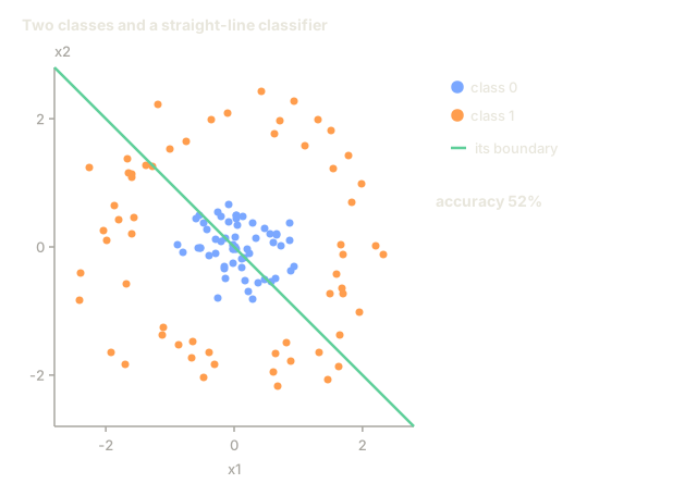
I've watched this happen more times than I can count. In classical ML, the representation of the data matters more than the choice of algorithm. A house price model with "square footage" and "number of bedrooms" will beat a model with "address as a raw string" no matter how sophisticated the learner is. The algorithm can only work with what you give it.
Feature engineering is the process of transforming raw data into representations that make patterns easier for models to find. Feature selection is the process of throwing away features that add noise without adding signal. Together, they are the single highest-impact activity in classical ML.
The Concept
The Feature Pipeline

Numerical Features
Raw numbers are rarely model-ready. Common transforms:
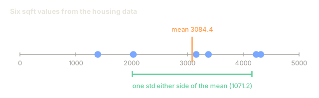
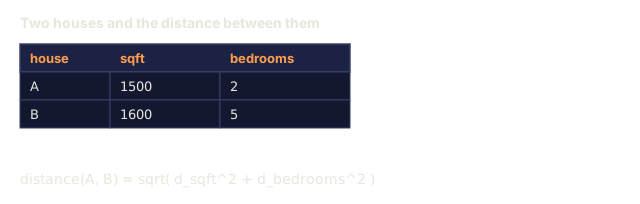
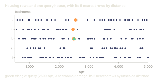
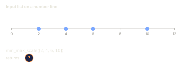
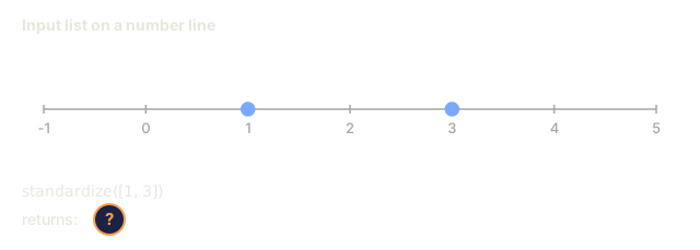
Scaling: Put features on the same range so distance-based algorithms (K-Means, KNN, SVM) treat all features equally. Min-max scaling maps to [0, 1]. Standardization (z-score) maps to mean=0, std=1.
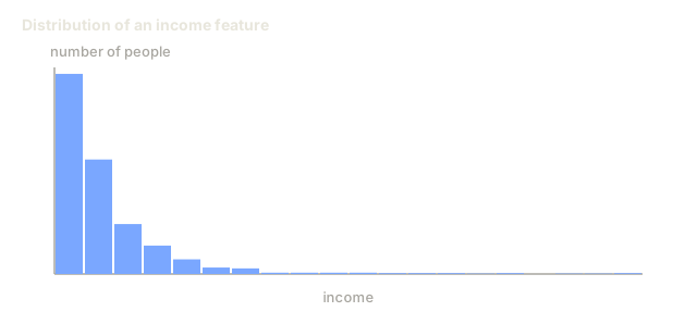
Log transform: Compresses right-skewed distributions (income, population, word counts). Turns multiplicative relationships into additive ones.
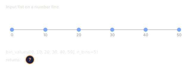
Binning: Converts continuous values into categories. Useful when the relationship between feature and target is non-linear but step-wise (e.g., age groups).
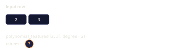
Polynomial features: Creates x^2, x^3, x1*x2 terms. Lets linear models capture non-linear relationships at the cost of more features.
Categorical Features
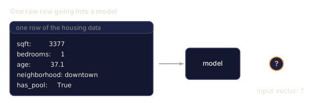
Models need numbers. Categories need encoding.
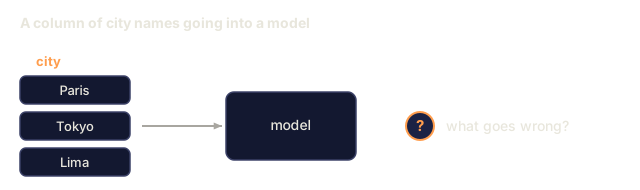
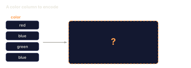
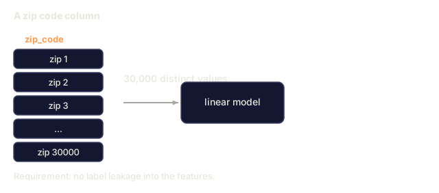
One-hot encoding: Creates a binary column for each category. "color = red/blue/green" becomes three columns: is_red, is_blue, is_green. Works well for low-cardinality features but explodes with many categories.
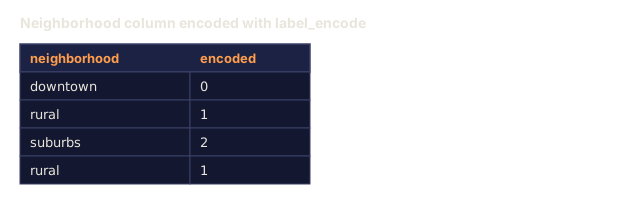
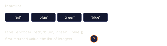
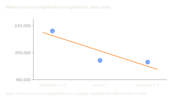
Label encoding: Maps each category to an integer: red=0, blue=1, green=2. Introduces false ordering (the model might think green > blue > red). Only appropriate for tree-based models that split on individual values.
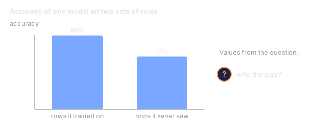
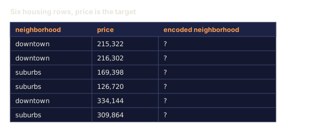
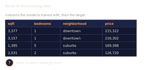
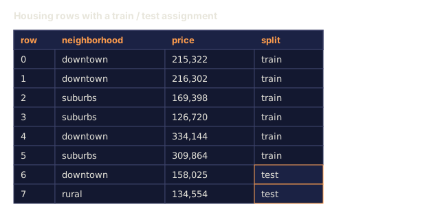
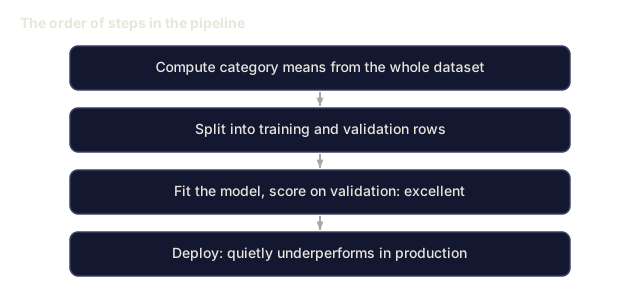
Target encoding: Replaces each category with the mean of the target variable for that category. Powerful but dangerous: high risk of data leakage. Must be computed only on training data and applied to test data.
Text Features
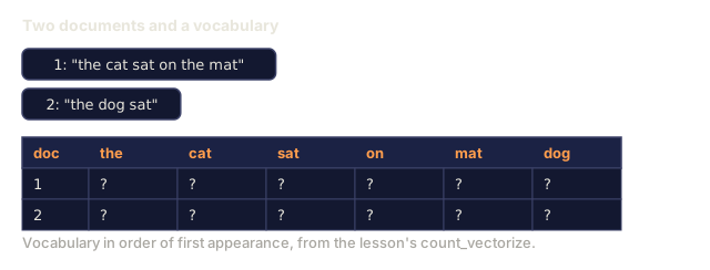
Count vectorizer: Counts how many times each word appears in a document. "the cat sat on the mat" becomes {the: 2, cat: 1, sat: 1, on: 1, mat: 1}.
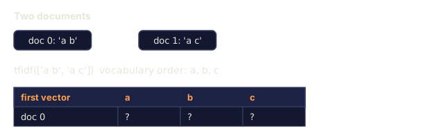
TF-IDF: Term Frequency-Inverse Document Frequency. Weighs words by how unique they are across documents. Common words like "the" get low weight. Rare, distinctive words get high weight.
TF(word, doc) = count(word in doc) / total words in doc
IDF(word) = log(total docs / docs containing word)
TF-IDF = TF * IDF
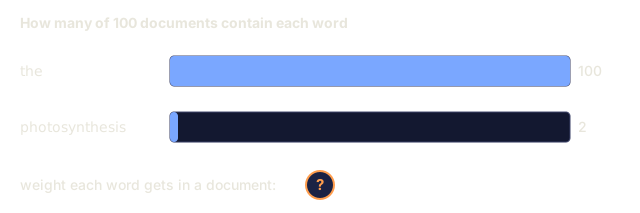
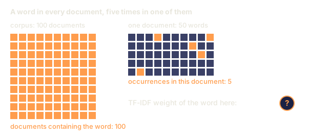
Example: across a 100-document corpus, "the" appears in all 100 documents and 5 times in one particular 50-word document. "photosynthesis" appears in only 2 of those documents, once in that same 50-word document.
TF-IDF("the")            = (5/50) * log(100/100) = 0.10 * 0    = 0.0
TF-IDF("photosynthesis") = (1/50) * log(100/2)   = 0.02 * 3.91 = 0.078
"the" shows up five times more often in the document, but contributes nothing: it appears in every document, so it carries no information about what makes this document distinctive. "photosynthesis" is rare across the corpus, so its single occurrence still pulls the document's vector toward the topic it is actually about.
Missing Values
Real data has holes. Strategies:
- Drop rows: Only when missing data is rare and random
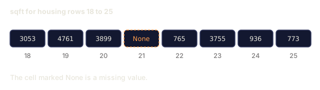
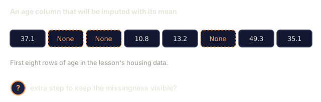
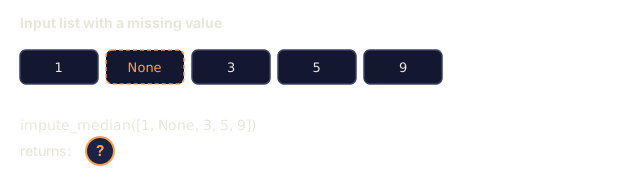
- Mean/median imputation: Simple, preserves distribution shape (median is more robust to outliers)
- Mode imputation: For categorical features
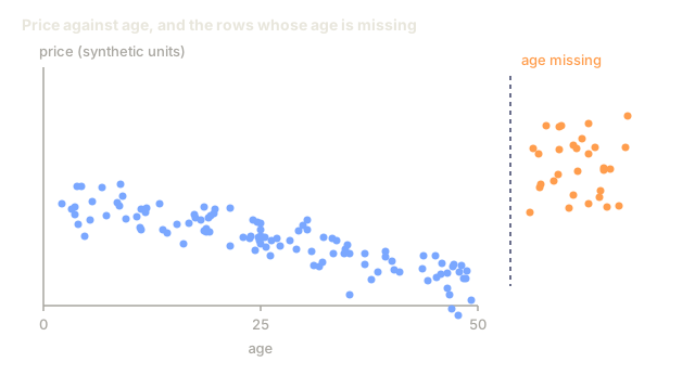
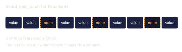
- Indicator column: Add a binary column "was_this_missing" before imputing. The fact that data is missing can itself be informative
- Forward/backward fill: For time series data
Feature Interaction
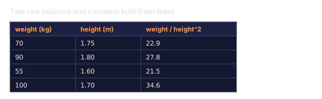
Feature interaction: the signal sometimes lives in the combination of two features, not in either one alone. "Height" and "weight" apart are less predictive than "BMI = weight / height^2" together. Interactions multiply the feature space fast, so pick them with domain knowledge instead of generating every possible pair.
Feature Selection
More features is not always better. Irrelevant features add noise, increase training time, and can cause overfitting.
Filter methods (pre-model):
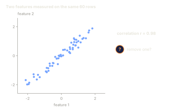
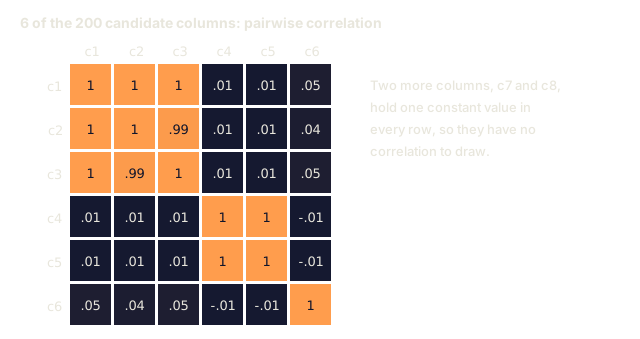
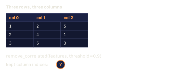
- Correlation: remove features highly correlated with each other (redundant)
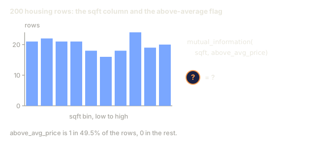
- Mutual information: measures how much knowing a feature reduces uncertainty about the target
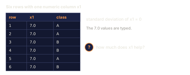
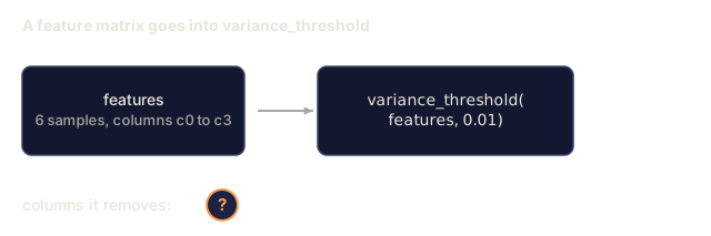
- Variance threshold: remove features that barely vary
Wrapper methods (model-based):
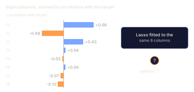
- L1 regularization (Lasso): drives irrelevant feature weights to exactly zero
- Recursive feature elimination: train, remove least important feature, repeat
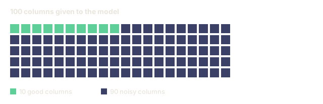
Why selection matters: A model with 10 good features will usually outperform a model with 10 good features and 90 noisy ones. The noisy features give the model opportunities to overfit on training data patterns that do not generalize.
Build It
Step 1: Numerical transforms from scratch
import math


def min_max_scale(values):
    min_val = min(values)
    max_val = max(values)
    if max_val == min_val:
        return [0.0] * len(values)
    return [(v - min_val) / (max_val - min_val) for v in values]


def standardize(values):
    n = len(values)
    mean = sum(values) / n
    variance = sum((v - mean) ** 2 for v in values) / n
    std = math.sqrt(variance) if variance > 0 else 1.0
    return [(v - mean) / std for v in values]


def log_transform(values):
    return [math.log(v + 1) for v in values]


def bin_values(values, n_bins=5):
    min_val = min(values)
    max_val = max(values)
    bin_width = (max_val - min_val) / n_bins
    if bin_width == 0:
        return [0] * len(values)
    result = []
    for v in values:
        bin_idx = int((v - min_val) / bin_width)
        bin_idx = min(bin_idx, n_bins - 1)
        result.append(bin_idx)
    return result


def polynomial_features(row, degree=2):
    n = len(row)
    result = list(row)
    if degree >= 2:
        for i in range(n):
            result.append(row[i] ** 2)
        for i in range(n):
            for j in range(i + 1, n):
                result.append(row[i] * row[j])
    return result
Step 2: Categorical encoding from scratch
def one_hot_encode(values):
    categories = sorted(set(values))
    cat_to_idx = {cat: i for i, cat in enumerate(categories)}
    n_cats = len(categories)

    encoded = []
    for v in values:
        row = [0] * n_cats
        row[cat_to_idx[v]] = 1
        encoded.append(row)

    return encoded, categories


def label_encode(values):
    categories = sorted(set(values))
    cat_to_int = {cat: i for i, cat in enumerate(categories)}
    return [cat_to_int[v] for v in values], cat_to_int


def target_encode(feature_values, target_values, smoothing=10):
    global_mean = sum(target_values) / len(target_values)

    category_stats = {}
    for feat, target in zip(feature_values, target_values):
        if feat not in category_stats:
            category_stats[feat] = {"sum": 0.0, "count": 0}
        category_stats[feat]["sum"] += target
        category_stats[feat]["count"] += 1

    encoding = {}
    for cat, stats in category_stats.items():
        cat_mean = stats["sum"] / stats["count"]
        weight = stats["count"] / (stats["count"] + smoothing)
        encoding[cat] = weight * cat_mean + (1 - weight) * global_mean

    return [encoding[v] for v in feature_values], encoding
Step 3: Text features from scratch
def count_vectorize(documents):
    vocab = {}
    idx = 0
    for doc in documents:
        for word in doc.lower().split():
            if word not in vocab:
                vocab[word] = idx
                idx += 1

    vectors = []
    for doc in documents:
        vec = [0] * len(vocab)
        for word in doc.lower().split():
            vec[vocab[word]] += 1
        vectors.append(vec)

    return vectors, vocab


def tfidf(documents):
    n_docs = len(documents)

    vocab = {}
    idx = 0
    for doc in documents:
        for word in doc.lower().split():
            if word not in vocab:
                vocab[word] = idx
                idx += 1

    doc_freq = {}
    for doc in documents:
        seen = set()
        for word in doc.lower().split():
            if word not in seen:
                doc_freq[word] = doc_freq.get(word, 0) + 1
                seen.add(word)

    vectors = []
    for doc in documents:
        words = doc.lower().split()
        word_count = len(words)
        tf_map = {}
        for word in words:
            tf_map[word] = tf_map.get(word, 0) + 1

        vec = [0.0] * len(vocab)
        for word, count in tf_map.items():
            tf = count / word_count
            idf = math.log(n_docs / doc_freq[word])
            vec[vocab[word]] = tf * idf
        vectors.append(vec)

    return vectors, vocab
Step 4: Missing value imputation from scratch
def impute_mean(values):
    present = [v for v in values if v is not None]
    if not present:
        return [0.0] * len(values), 0.0
    mean = sum(present) / len(present)
    return [v if v is not None else mean for v in values], mean


def impute_median(values):
    present = sorted(v for v in values if v is not None)
    if not present:
        return [0.0] * len(values), 0.0
    n = len(present)
    if n % 2 == 0:
        median = (present[n // 2 - 1] + present[n // 2]) / 2
    else:
        median = present[n // 2]
    return [v if v is not None else median for v in values], median


def impute_mode(values):
    present = [v for v in values if v is not None]
    if not present:
        return values, None
    counts = {}
    for v in present:
        counts[v] = counts.get(v, 0) + 1
    mode = max(counts, key=counts.get)
    return [v if v is not None else mode for v in values], mode


def add_missing_indicator(values):
    return [0 if v is not None else 1 for v in values]
Step 5: Feature selection from scratch
def correlation(x, y):
    n = len(x)
    mean_x = sum(x) / n
    mean_y = sum(y) / n
    cov = sum((xi - mean_x) * (yi - mean_y) for xi, yi in zip(x, y)) / n
    std_x = math.sqrt(sum((xi - mean_x) ** 2 for xi in x) / n)
    std_y = math.sqrt(sum((yi - mean_y) ** 2 for yi in y) / n)
    if std_x == 0 or std_y == 0:
        return 0.0
    return cov / (std_x * std_y)


def mutual_information(feature, target, n_bins=10):
    feat_min = min(feature)
    feat_max = max(feature)
    bin_width = (feat_max - feat_min) / n_bins if feat_max != feat_min else 1.0
    feat_binned = [
        min(int((f - feat_min) / bin_width), n_bins - 1) for f in feature
    ]

    n = len(feature)
    target_classes = sorted(set(target))

    feat_bins = sorted(set(feat_binned))
    p_feat = {}
    for b in feat_bins:
        p_feat[b] = feat_binned.count(b) / n

    p_target = {}
    for t in target_classes:
        p_target[t] = target.count(t) / n

    mi = 0.0
    for b in feat_bins:
        for t in target_classes:
            joint_count = sum(
                1 for fb, tv in zip(feat_binned, target) if fb == b and tv == t
            )
            p_joint = joint_count / n
            if p_joint > 0:
                mi += p_joint * math.log(p_joint / (p_feat[b] * p_target[t]))

    return mi


def variance_threshold(features, threshold=0.01):
    n_features = len(features[0])
    n_samples = len(features)
    selected = []

    for j in range(n_features):
        col = [features[i][j] for i in range(n_samples)]
        mean = sum(col) / n_samples
        var = sum((v - mean) ** 2 for v in col) / n_samples
        if var >= threshold:
            selected.append(j)

    return selected


def remove_correlated(features, threshold=0.9):
    n_features = len(features[0])
    n_samples = len(features)

    to_remove = set()
    for i in range(n_features):
        if i in to_remove:
            continue
        col_i = [features[r][i] for r in range(n_samples)]
        for j in range(i + 1, n_features):
            if j in to_remove:
                continue
            col_j = [features[r][j] for r in range(n_samples)]
            corr = abs(correlation(col_i, col_j))
            if corr >= threshold:
                to_remove.add(j)

    return [i for i in range(n_features) if i not in to_remove]
Step 6: Full pipeline and demo
import random


def make_housing_data(n=200, seed=42):
    random.seed(seed)
    data = []
    for _ in range(n):
        sqft = random.uniform(500, 5000)
        bedrooms = random.choice([1, 2, 3, 4, 5])
        age = random.uniform(0, 50)
        neighborhood = random.choice(["downtown", "suburbs", "rural"])
        has_pool = random.choice([True, False])

        sqft_with_missing = sqft if random.random() > 0.05 else None
        age_with_missing = age if random.random() > 0.08 else None

        price = (
            50 * sqft
            + 20000 * bedrooms
            - 1000 * age
            + (50000 if neighborhood == "downtown" else 10000 if neighborhood == "suburbs" else 0)
            + (15000 if has_pool else 0)
            + random.gauss(0, 20000)
        )

        data.append({
            "sqft": sqft_with_missing,
            "bedrooms": bedrooms,
            "age": age_with_missing,
            "neighborhood": neighborhood,
            "has_pool": has_pool,
            "price": price,
        })
    return data


if __name__ == "__main__":
    data = make_housing_data(200)

    print("=== Raw Data Sample ===")
    for row in data[:3]:
        print(f"  {row}")

    sqft_raw = [d["sqft"] for d in data]
    age_raw = [d["age"] for d in data]
    prices = [d["price"] for d in data]

    print("\n=== Missing Value Handling ===")
    sqft_missing = sum(1 for v in sqft_raw if v is None)
    age_missing = sum(1 for v in age_raw if v is None)
    print(f"  sqft missing: {sqft_missing}/{len(sqft_raw)}")
    print(f"  age missing: {age_missing}/{len(age_raw)}")

    sqft_indicator = add_missing_indicator(sqft_raw)
    age_indicator = add_missing_indicator(age_raw)
    sqft_imputed, sqft_fill = impute_median(sqft_raw)
    age_imputed, age_fill = impute_mean(age_raw)
    print(f"  sqft filled with median: {sqft_fill:.0f}")
    print(f"  age filled with mean: {age_fill:.1f}")

    print("\n=== Numerical Transforms ===")
    sqft_scaled = standardize(sqft_imputed)
    age_scaled = min_max_scale(age_imputed)
    sqft_log = log_transform(sqft_imputed)
    age_binned = bin_values(age_imputed, n_bins=5)
    print(f"  sqft standardized: mean={sum(sqft_scaled)/len(sqft_scaled):.4f}, std={math.sqrt(sum(v**2 for v in sqft_scaled)/len(sqft_scaled)):.4f}")
    print(f"  age min-max: [{min(age_scaled):.2f}, {max(age_scaled):.2f}]")
    print(f"  age bins: {sorted(set(age_binned))}")

    print("\n=== Categorical Encoding ===")
    neighborhoods = [d["neighborhood"] for d in data]

    ohe, ohe_cats = one_hot_encode(neighborhoods)
    print(f"  One-hot categories: {ohe_cats}")
    print(f"  Sample encoding: {neighborhoods[0]} -> {ohe[0]}")

    le, le_map = label_encode(neighborhoods)
    print(f"  Label encoding map: {le_map}")

    te, te_map = target_encode(neighborhoods, prices, smoothing=10)
    print(f"  Target encoding: {({k: round(v) for k, v in te_map.items()})}")

    print("\n=== Text Features ===")
    descriptions = [
        "large modern house with pool",
        "small cozy cottage near downtown",
        "spacious family home with large yard",
        "modern apartment downtown with view",
        "rustic cabin in rural area",
    ]
    cv, cv_vocab = count_vectorize(descriptions)
    print(f"  Vocabulary size: {len(cv_vocab)}")
    print(f"  Doc 0 non-zero features: {sum(1 for v in cv[0] if v > 0)}")

    tf, tf_vocab = tfidf(descriptions)
    print(f"  TF-IDF vocabulary size: {len(tf_vocab)}")
    top_words = sorted(tf_vocab.keys(), key=lambda w: tf[0][tf_vocab[w]], reverse=True)[:3]
    print(f"  Doc 0 top TF-IDF words: {top_words}")

    print("\n=== Polynomial Features ===")
    sample_row = [sqft_scaled[0], age_scaled[0]]
    poly = polynomial_features(sample_row, degree=2)
    print(f"  Input: {[round(v, 4) for v in sample_row]}")
    print(f"  Polynomial: {[round(v, 4) for v in poly]}")
    print(f"  Features: [x1, x2, x1^2, x2^2, x1*x2]")

    print("\n=== Feature Selection ===")
    feature_matrix = [
        [sqft_scaled[i], age_scaled[i], float(sqft_indicator[i]), float(age_indicator[i])]
        + ohe[i]
        for i in range(len(data))
    ]

    print(f"  Total features: {len(feature_matrix[0])}")

    surviving_var = variance_threshold(feature_matrix, threshold=0.01)
    print(f"  After variance threshold (0.01): {len(surviving_var)} features kept")

    surviving_corr = remove_correlated(feature_matrix, threshold=0.9)
    print(f"  After correlation filter (0.9): {len(surviving_corr)} features kept")

    binary_prices = [1 if p > sum(prices) / len(prices) else 0 for p in prices]
    print("\n  Mutual information with target:")
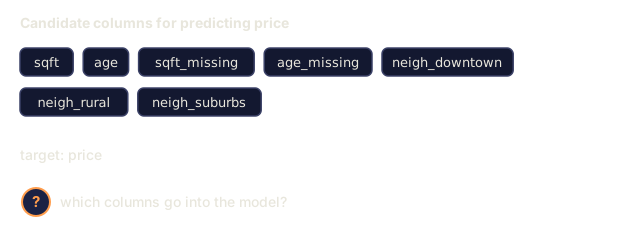
    feature_names = ["sqft", "age", "sqft_missing", "age_missing"] + [f"neigh_{c}" for c in ohe_cats]
    for j in range(len(feature_matrix[0])):
        col = [feature_matrix[i][j] for i in range(len(feature_matrix))]
        mi = mutual_information(col, binary_prices, n_bins=10)
        print(f"    {feature_names[j]}: MI={mi:.4f}")

    print("\n  Correlation with price:")
    for j in range(len(feature_matrix[0])):
        col = [feature_matrix[i][j] for i in range(len(feature_matrix))]
        corr = correlation(col, prices)
        print(f"    {feature_names[j]}: r={corr:.4f}")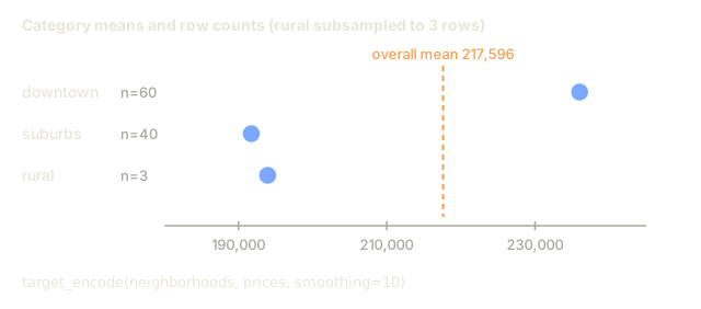
Use It
With scikit-learn, these transforms are composable pipelines:
from sklearn.preprocessing import StandardScaler, OneHotEncoder, PolynomialFeatures
from sklearn.impute import SimpleImputer
from sklearn.feature_extraction.text import TfidfVectorizer
from sklearn.feature_selection import mutual_info_classif, VarianceThreshold
from sklearn.compose import ColumnTransformer
from sklearn.pipeline import Pipeline

numeric_pipe = Pipeline([
    ("imputer", SimpleImputer(strategy="median")),
    ("scaler", StandardScaler()),
])

categorical_pipe = Pipeline([
    ("encoder", OneHotEncoder(sparse_output=False)),
])

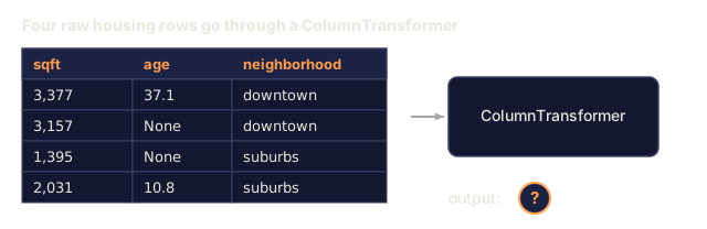
preprocessor = ColumnTransformer([
    ("num", numeric_pipe, ["sqft", "age"]),
    ("cat", categorical_pipe, ["neighborhood"]),
])
The from-scratch versions show exactly what happens inside each transform. The library versions add edge-case handling, sparse matrix support, and pipeline composition, but the math is the same.
Ship It
This lesson produces:
outputs/prompt-feature-engineer.md, a prompt for systematically engineering features from raw data
The biggest mistake I've seen with target encoding isn't in the formula, it's in the order of operations. Compute the category means on the full dataset, including rows that will later become your test set, and validation scores look fantastic. Ship that model and watch it underperform quietly in production. The encoding was fit on data that included the rows it was later validated against, so those inflated scores were measuring leakage, not skill. Genuinely held-out data doesn't return the favor. Fit the encoding on the training fold only, every time, even when it feels like you're throwing away information.
If I had a week to spend improving a mediocre tabular model, I would spend all five days on features before I touched a single hyperparameter. That bet has paid off far more often than the reverse.
Exercises
- Add robust scaling (using median and interquartile range instead of mean and standard deviation) to the numerical transforms. Compare it to standard scaling on data with extreme outliers.
- Implement leave-one-out target encoding: for each row, compute the target mean excluding that row's own target value. Show how this reduces overfitting compared to naive target encoding.
- Build an automated feature selection pipeline that combines variance threshold, correlation filtering, and mutual information ranking. Apply it to the housing dataset and compare model performance (use a simple linear regression) with all features vs selected features.
Key Terms
| Term | What people say | What it actually means |
|---|---|---|
| Feature engineering | "Making new columns" | Transforming raw data into representations that expose patterns to the model |
| Standardization | "Making it normal" | Subtracting the mean and dividing by standard deviation so the feature has mean=0 and std=1 |
| One-hot encoding | "Making dummy variables" | Creating one binary column per category, where exactly one column is 1 for each row |
| Target encoding | "Using the answer to encode" | Replacing each category with the average target value for that category, with smoothing to prevent overfitting |
| TF-IDF | "Fancy word counts" | Term Frequency times Inverse Document Frequency: words weighted by how distinctive they are across the corpus |
| Imputation | "Filling in blanks" | Replacing missing values with estimated values (mean, median, mode, or model-predicted) |
| Feature selection | "Throwing out bad columns" | Removing features that add noise or redundancy, keeping only those with signal about the target |
| Mutual information | "How much one thing tells you about another" | A measure of the reduction in uncertainty about variable Y gained by observing variable X |
| Data leakage | "Accidentally cheating" | Using information during training that would not be available at prediction time, giving falsely optimistic results |
Further Reading
- Feature Engineering and Selection (Max Kuhn & Kjell Johnson) - free online book covering the full landscape of feature engineering
- scikit-learn Preprocessing Guide - practical reference for all standard transforms
- Target Encoding Done Right (Micci-Barreca, 2001) - the original paper on target encoding with smoothing
Code
- features.py (python, 392 lines)