Feature Selection
More features isn't better. The right features are.
Learning Objectives
- Implement filter methods (variance threshold, mutual information) and wrapper methods (RFE, forward selection) from scratch
- Explain why mutual information captures nonlinear feature-target relationships that correlation misses
- Compare L1 regularization (embedded selection) with RFE (wrapper selection) and evaluate their computational tradeoffs
- Build a feature selection pipeline that combines multiple methods and demonstrate improved generalization on held-out data
The Problem
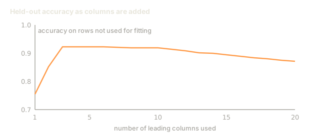
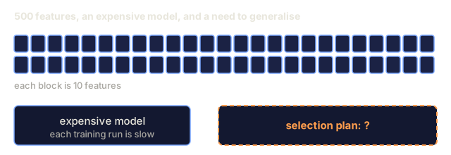
Say you have 500 features. The model trains slowly, overfits constantly, and nobody on the team can explain what it actually learned. You throw more features at it hoping that helps. It gets worse.
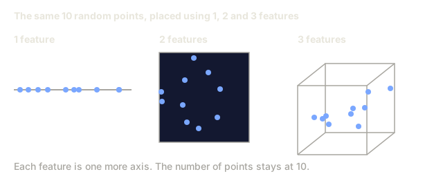
That's the curse of dimensionality doing its job. As the feature count grows, the feature space's volume explodes. Data points get sparser. Distances between them start to converge toward meaningless. Finding a real pattern in that emptiness takes exponentially more data than you have. Every noise feature you added along the way drowns out the signal from the ones that actually mattered. Overfitting stops being a risk and becomes the default.
Feature selection fixes that by cutting what doesn't help: strip the noise, remove the redundancy, keep only the features carrying real information about the target. The payoff is faster training, better generalization, and a model you can actually explain to someone else.
The goal isn't to use all the information available. It's to use the right information.
The Concept
Three Categories of Feature Selection
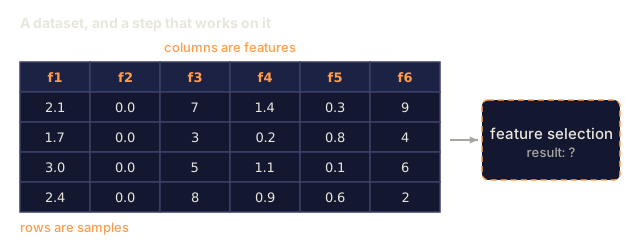
Feature selection is choosing which subset of your available features a model should actually use, and discarding the rest. Every method for doing that falls into one of three categories:

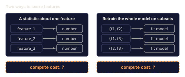
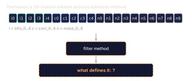
Filter methods score each feature on its own, using a statistical measure and no model at all. That makes them fast, but blind to how features interact with each other.
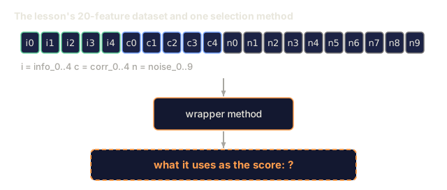
Wrapper methods go the other way: they train an actual model on different feature subsets and use its performance as the score. Results are usually better, at the cost of retraining the model over and over.
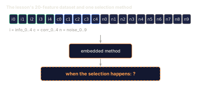
Embedded methods fold selection into training itself, rather than running it as a separate step. L1 regularization drives irrelevant weights to zero as it fits; decision trees split on whichever feature is most useful at each node. Either way, you get the selection for free from a model you were already training.
Variance Threshold
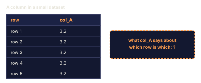
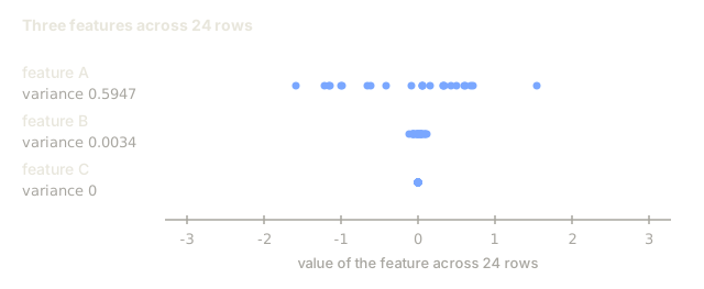
The simplest filter there is. If a feature barely moves across your samples, it isn't carrying much information to begin with.
Take a feature that's 0.0 for 999 out of 1000 samples. Its variance is essentially zero, and no model can use a value that never changes to tell one class from another. Remove it.
variance(x) = mean((x - mean(x))^2)
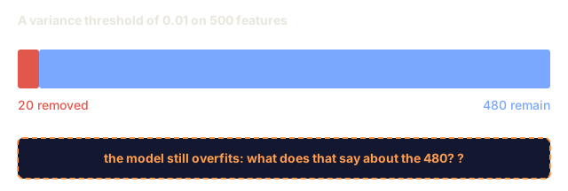
Pick a threshold (0.01 is a common start) and drop every feature whose variance falls below it. That clears out constant and near-constant features without even glancing at the target.
When to use it: as a cheap preprocessing step before running anything heavier. It catches the obviously useless features at close to zero cost.
Limitation: high variance doesn't guarantee a feature is useful, only that it isn't constant. Variance threshold is necessary, not sufficient.
Mutual Information
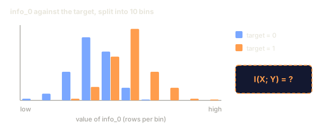
Mutual information measures how much knowing feature X reduces your uncertainty about target Y.
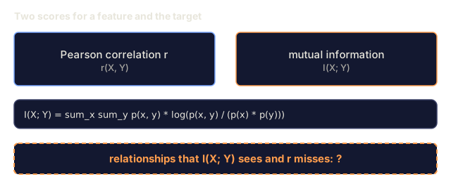
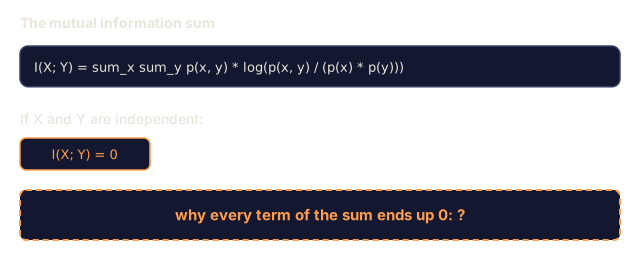
I(X; Y) = sum_x sum_y p(x, y) * log(p(x, y) / (p(x) * p(y)))
If X and Y are independent, p(x, y) = p(x) * p(y), the log term collapses to zero, and I(X; Y) = 0. The more X tells you about Y, the higher the score climbs.
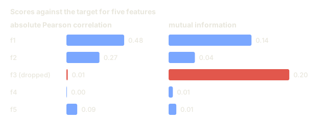
Its advantage over correlation: mutual information catches nonlinear relationships too. A feature can sit at zero correlation with the target and still carry a high mutual information score, because the real relationship is quadratic or periodic rather than linear.
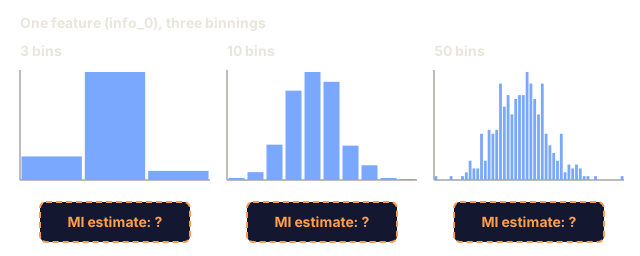
For continuous features, discretize into bins first (histogram-based estimation). The number of bins affects the estimate: too few and you lose information, too many and you add noise. A common choice is sqrt(n) bins, or Sturges' rule, 1 + log2(n).

Recursive Feature Elimination (RFE)
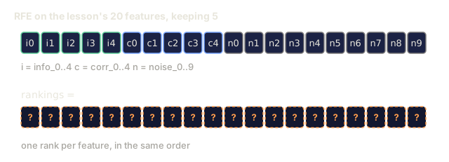
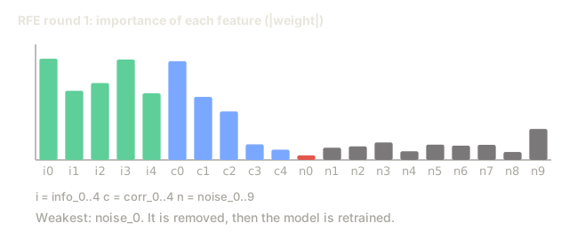
RFE is a wrapper method that leans on a model's own feature importance to prune, one round at a time:
- Train the model with all features
- Rank features by importance (coefficients for linear models, impurity reduction for trees)
- Remove the least important feature(s)
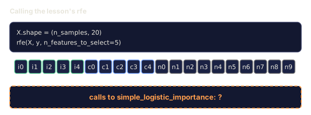
- Repeat until the desired number of features remains

Because the model sees every remaining feature at once, RFE picks up on interactions that filter methods miss entirely: remove one feature and the importance of the others shifts, and RFE lets the model reassess on every round instead of judging everything up front.
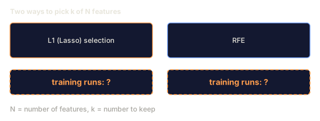
The cost is real: you're training the model N minus target times. With 500 features and a target of 10, that's 490 training runs, which gets slow fast for anything expensive to train. Removing a chunk of the bottom features per round (say, the bottom 10%) instead of one at a time is the usual fix.
L1 (Lasso) Regularization
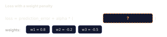
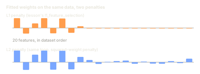
L1 regularization adds the sum of the absolute weight values to the loss function:
loss = prediction_error + alpha * sum(|w_i|)
The alpha parameter sets how aggressively features get pruned: push it higher and more weights land at exactly zero.
Why exactly zero, and not just small? The L1 penalty carves out a diamond-shaped constraint region in weight space, and the optimal solution tends to land on a corner of that diamond, where one or more weights are exactly zero. Ridge (L2) carves out a circle instead, so weights shrink toward zero but almost never actually hit it.
That's embedded selection in practice: the model decides which features to ignore as it trains, and a feature with zero weight is gone in every way that matters.
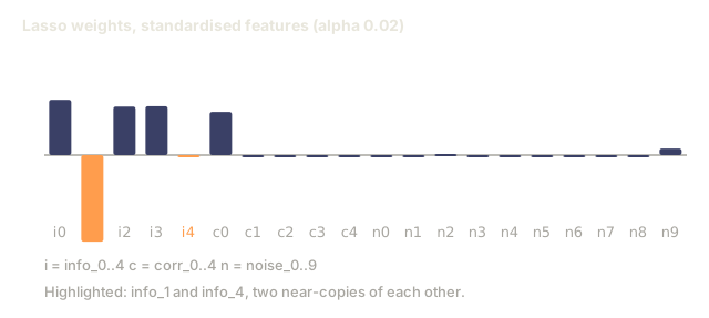
Advantages: one training run, handles correlated features by picking one and zeroing the rest, and it's already built into most linear model libraries.
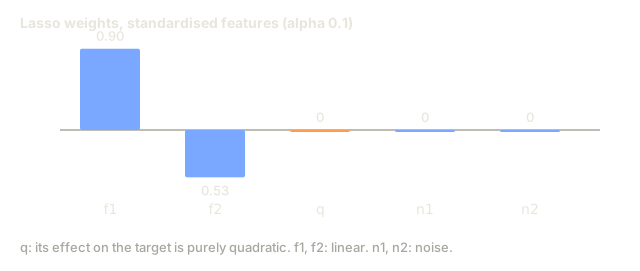
Limitation: it only works for linear models. Nonlinear feature importance is invisible to it.
Tree-Based Feature Importance
Decision trees and their ensembles (random forests, gradient boosting) rank features as a side effect of how they're built. Every split reduces impurity (Gini or entropy for classification, variance for regression), and whichever features drive the biggest reductions come out looking most important.
For a random forest with T trees:
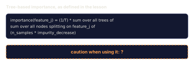
importance(feature_j) = (1/T) * sum over all trees of
    sum over all nodes splitting on feature_j of
        (n_samples * impurity_decrease)
That gives a normalized importance score per feature, and it picks up nonlinear relationships and interactions without any extra work.
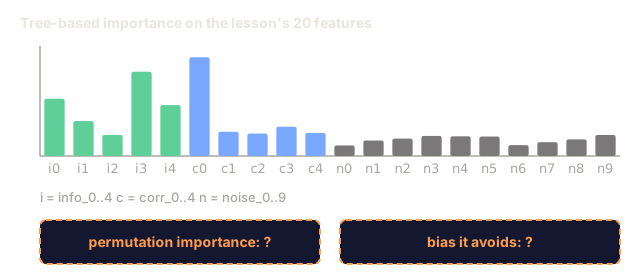
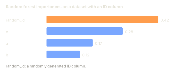
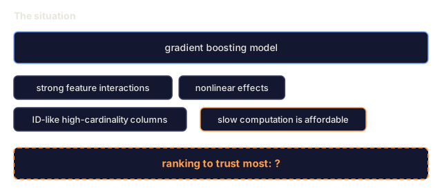
Caution: tree-based importance is biased toward high-cardinality features, ones with lots of unique values. A random ID column will look important because it can split every sample perfectly, even though it's meaningless. Run permutation importance as a sanity check before trusting the ranking.
Permutation Importance
A model-agnostic method that doesn't care what's inside the model:
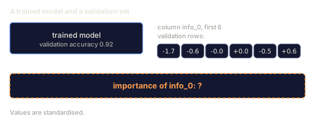
- Train the model and record baseline performance on validation data
- For each feature, shuffle its values randomly and measure the drop in performance
- The bigger the drop, the more important the feature
Shuffle a feature and performance barely moves? The model wasn't leaning on it. Performance collapses instead, and that feature was doing real work.
It sidesteps the cardinality bias that trips up tree-based importance, but it's slow: one full evaluation per feature, repeated several times for stability.
Comparison Table
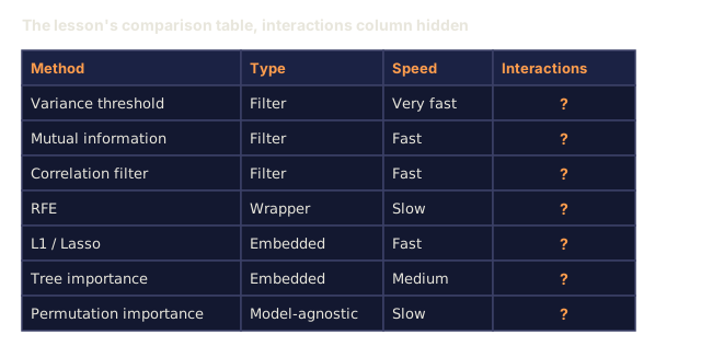
| Method | Type | Speed | Nonlinear | Feature Interactions |
|---|---|---|---|---|
| Variance threshold | Filter | Very fast | No | No |
| Mutual information | Filter | Fast | Yes | No |
| Correlation filter | Filter | Fast | No | No |
| RFE | Wrapper | Slow | Depends on model | Yes |
| L1 / Lasso | Embedded | Fast | No (linear) | No |
| Tree importance | Embedded | Medium | Yes | Yes |
| Permutation importance | Model-agnostic | Slow | Yes | Yes |
Decision Flowchart


Build It
Step 1: Generate synthetic data with known feature structure
import numpy as np


def make_feature_selection_data(n_samples=500, seed=42):
    rng = np.random.RandomState(seed)

    x1 = rng.randn(n_samples)
    x2 = rng.randn(n_samples)
    x3 = rng.randn(n_samples)
    x4 = x1 + 0.1 * rng.randn(n_samples)
    x5 = x2 + 0.1 * rng.randn(n_samples)

    informative = np.column_stack([x1, x2, x3, x4, x5])

    correlated = np.column_stack([
        x1 * 0.9 + 0.1 * rng.randn(n_samples),
        x2 * 0.8 + 0.2 * rng.randn(n_samples),
        x3 * 0.7 + 0.3 * rng.randn(n_samples),
        x1 * 0.5 + x2 * 0.5 + 0.1 * rng.randn(n_samples),
        x2 * 0.6 + x3 * 0.4 + 0.1 * rng.randn(n_samples),
    ])

    noise = rng.randn(n_samples, 10) * 0.5

    X = np.hstack([informative, correlated, noise])
    y = (2 * x1 - 1.5 * x2 + x3 + 0.5 * rng.randn(n_samples) > 0).astype(int)

    feature_names = (
        [f"info_{i}" for i in range(5)]
        + [f"corr_{i}" for i in range(5)]
        + [f"noise_{i}" for i in range(10)]
    )

    return X, y, feature_names
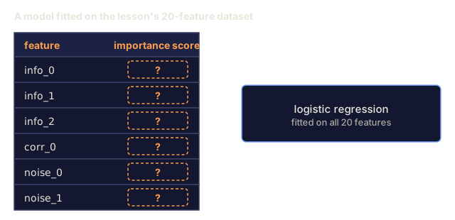
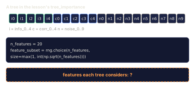
We built this with the ground truth baked in: features 0-4 are informative (features 3 and 4 are just correlated copies of 0 and 1), features 5-9 correlate with the informative ones, and features 10-19 are pure noise. Any selection method worth using should rank 0-4 at the top and 10-19 at the bottom.
Step 2: Variance threshold
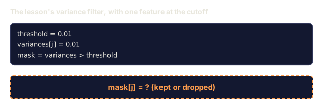
def variance_threshold(X, threshold=0.01):
    variances = np.var(X, axis=0)
    mask = variances > threshold
    return mask, variances
Step 3: Mutual information (discrete)
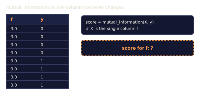
def discretize(x, n_bins=10):
    min_val, max_val = x.min(), x.max()
    if max_val == min_val:
        return np.zeros_like(x, dtype=int)
    bin_edges = np.linspace(min_val, max_val, n_bins + 1)
    binned = np.digitize(x, bin_edges[1:-1])
    return binned


def mutual_information(X, y, n_bins=10):
    n_samples, n_features = X.shape
    mi_scores = np.zeros(n_features)

    y_vals, y_counts = np.unique(y, return_counts=True)
    p_y = y_counts / n_samples

    for f in range(n_features):
        x_binned = discretize(X[:, f], n_bins)
        x_vals, x_counts = np.unique(x_binned, return_counts=True)
        p_x = dict(zip(x_vals, x_counts / n_samples))

        mi = 0.0
        for xv in x_vals:
            for yi, yv in enumerate(y_vals):
                joint_mask = (x_binned == xv) & (y == yv)
                p_xy = np.sum(joint_mask) / n_samples
                if p_xy > 0:
                    mi += p_xy * np.log(p_xy / (p_x[xv] * p_y[yi]))
        mi_scores[f] = mi

    return mi_scores
Step 4: Recursive Feature Elimination
def simple_logistic_importance(X, y, lr=0.1, epochs=100):
    n_samples, n_features = X.shape
    w = np.zeros(n_features)
    b = 0.0

    for _ in range(epochs):
        z = X @ w + b
        pred = 1.0 / (1.0 + np.exp(-np.clip(z, -500, 500)))
        error = pred - y
        w -= lr * (X.T @ error) / n_samples
        b -= lr * np.mean(error)

    return w, b


def rfe(X, y, n_features_to_select=5, lr=0.1, epochs=100):
    n_total = X.shape[1]
    remaining = list(range(n_total))
    rankings = np.ones(n_total, dtype=int)
    rank = n_total

    while len(remaining) > n_features_to_select:
        X_subset = X[:, remaining]
        w, _ = simple_logistic_importance(X_subset, y, lr, epochs)
        importances = np.abs(w)

        least_idx = np.argmin(importances)
        original_idx = remaining[least_idx]
        rankings[original_idx] = rank
        rank -= 1
        remaining.pop(least_idx)

    for idx in remaining:
        rankings[idx] = 1

    selected_mask = rankings == 1
    return selected_mask, rankings
Step 5: L1 feature selection
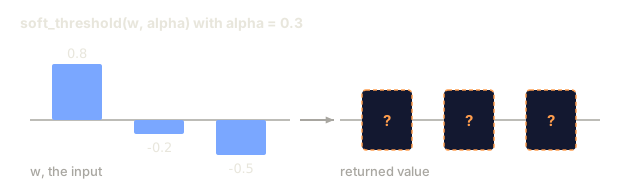
def soft_threshold(w, alpha):
    return np.sign(w) * np.maximum(np.abs(w) - alpha, 0)


def l1_feature_selection(X, y, alpha=0.1, lr=0.01, epochs=500):
    n_samples, n_features = X.shape
    w = np.zeros(n_features)
    b = 0.0

    for _ in range(epochs):
        z = X @ w + b
        pred = 1.0 / (1.0 + np.exp(-np.clip(z, -500, 500)))
        error = pred - y

        gradient_w = (X.T @ error) / n_samples
        gradient_b = np.mean(error)

        w -= lr * gradient_w
        w = soft_threshold(w, lr * alpha)
        b -= lr * gradient_b

    selected_mask = np.abs(w) > 1e-6
    return selected_mask, w
Step 6: Tree-based importance (simple decision tree)
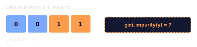
def gini_impurity(y):
    if len(y) == 0:
        return 0.0
    classes, counts = np.unique(y, return_counts=True)
    probs = counts / len(y)
    return 1.0 - np.sum(probs ** 2)


def best_split(X, y, feature_idx):
    values = np.unique(X[:, feature_idx])
    if len(values) <= 1:
        return None, -1.0

    best_threshold = None
    best_gain = -1.0
    parent_gini = gini_impurity(y)
    n = len(y)

    for i in range(len(values) - 1):
        threshold = (values[i] + values[i + 1]) / 2.0
        left_mask = X[:, feature_idx] <= threshold
        right_mask = ~left_mask

        n_left = np.sum(left_mask)
        n_right = np.sum(right_mask)

        if n_left == 0 or n_right == 0:
            continue

        gain = parent_gini - (n_left / n) * gini_impurity(y[left_mask]) - (n_right / n) * gini_impurity(y[right_mask])

        if gain > best_gain:
            best_gain = gain
            best_threshold = threshold

    return best_threshold, best_gain


def tree_importance(X, y, n_trees=50, max_depth=5, seed=42):
    rng = np.random.RandomState(seed)
    n_samples, n_features = X.shape
    importances = np.zeros(n_features)

    for _ in range(n_trees):
        sample_idx = rng.choice(n_samples, size=n_samples, replace=True)
        feature_subset = rng.choice(n_features, size=max(1, int(np.sqrt(n_features))), replace=False)

        X_boot = X[sample_idx]
        y_boot = y[sample_idx]

        tree_imp = _build_tree_importance(X_boot, y_boot, feature_subset, max_depth)
        importances += tree_imp

    total = importances.sum()
    if total > 0:
        importances /= total

    return importances


def _build_tree_importance(X, y, feature_subset, max_depth, depth=0):
    n_features = X.shape[1]
    importances = np.zeros(n_features)

    if depth >= max_depth or len(np.unique(y)) <= 1 or len(y) < 4:
        return importances

    best_feature = None
    best_threshold = None
    best_gain = -1.0

    for f in feature_subset:
        threshold, gain = best_split(X, y, f)
        if gain > best_gain:
            best_gain = gain
            best_feature = f
            best_threshold = threshold

    if best_feature is None or best_gain <= 0:
        return importances

    importances[best_feature] += best_gain * len(y)

    left_mask = X[:, best_feature] <= best_threshold
    right_mask = ~left_mask

    importances += _build_tree_importance(X[left_mask], y[left_mask], feature_subset, max_depth, depth + 1)
    importances += _build_tree_importance(X[right_mask], y[right_mask], feature_subset, max_depth, depth + 1)

    return importances
Step 7: Run all methods and compare
The code file runs all five methods against the same synthetic dataset and prints a comparison table showing which features each one keeps.
Use It
With scikit-learn, feature selection is already built into the pipeline:
from sklearn.feature_selection import (
    VarianceThreshold,
    mutual_info_classif,
    RFE,
    SelectFromModel,
)
from sklearn.linear_model import Lasso, LogisticRegression
from sklearn.ensemble import RandomForestClassifier

vt = VarianceThreshold(threshold=0.01)
X_filtered = vt.fit_transform(X)

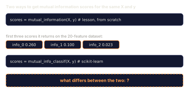
mi_scores = mutual_info_classif(X, y)
top_k = np.argsort(mi_scores)[-10:]

rfe_selector = RFE(LogisticRegression(), n_features_to_select=10)
rfe_selector.fit(X, y)
X_rfe = rfe_selector.transform(X)

lasso_selector = SelectFromModel(Lasso(alpha=0.01))
lasso_selector.fit(X, y)
X_lasso = lasso_selector.transform(X)

rf = RandomForestClassifier(n_estimators=100)
rf.fit(X, y)
importances = rf.feature_importances_
The from-scratch versions above show exactly what's happening inside each method. Variance threshold is just var(X, axis=0) with a mask applied on top. Mutual information is counting joint and marginal frequencies in a contingency table. RFE is a loop that trains, ranks, and prunes. L1 is gradient descent with a soft-thresholding step bolted on. Tree importance accumulates impurity reductions across every split. No magic. Just statistics and loops.
What sklearn adds on top: robustness (mutual_info_classif uses k-NN density estimation instead of binning), speed (C implementations under the hood), and pipeline integration you don't have to write yourself.
Ship It
This lesson produces outputs/skill-feature-selector.md, a quick-reference decision tree for picking the right feature selection method for a given dataset and model.
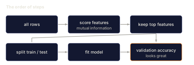
The mistake I see most with feature selection isn't picking the wrong method. It's running the method on the whole dataset before the train/test split.
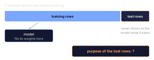
Say you compute mutual information scores, or fit RFE, on all your data, then split into train and test afterward. You just let the test set influence which features you kept. Every feature you selected is now biased toward doing well on data it technically hasn't seen yet, and your validation score is quietly lying to you about how the model will perform in production.
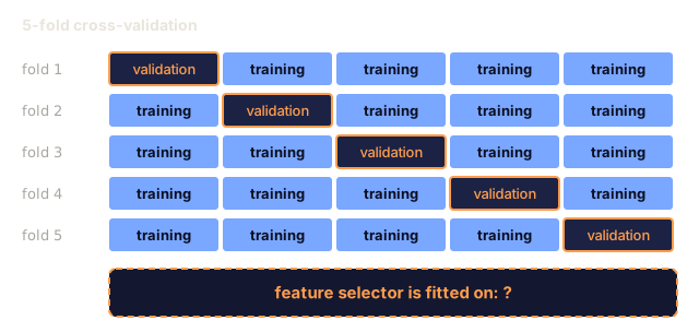
The fix is boring but non-negotiable: split first, fit your selector on the training fold only, then apply that same selection to the test fold without refitting. If you're doing k-fold cross-validation, the selection step belongs inside the fold loop, not outside it. I've watched this leak add two or three points of phantom accuracy to a validation score that evaporated the moment the model saw real data.
Exercises
-
Forward selection: implement the opposite of RFE. Start with zero features. At each step, add the feature that improves model performance the most. Stop when adding features no longer helps. Compare the selected features against RFE results. Which is faster? Which gives better results?
-
Stability selection: run L1 feature selection 50 times, each time on a random 80% subsample of the data, with slightly different alpha values. Count how often each feature is selected. Features selected in > 80% of runs are "stable." Compare stable features against single-run L1 selection. Which is more reliable?
-
Multicollinearity detection: compute the correlation matrix for all features. Implement a function that, given a correlation threshold (e.g., 0.9), removes one feature from each highly-correlated pair (keeping the one with higher mutual information with the target). Test on the synthetic dataset and verify it removes the redundant correlated features.
-
Feature selection pipeline: chain variance threshold, mutual information filter, and RFE into a single pipeline. First remove near-zero-variance features, then keep the top 50% by mutual information, then run RFE on the survivors. Compare this pipeline against running RFE alone on all features. Is the pipeline faster? Is it equally accurate?
-
Permutation importance from scratch: implement permutation importance. For each feature, shuffle its values 10 times, measure the average drop in F1 score. Compare the ranking against tree-based importance. Find cases where they disagree and explain why (hint: correlated features).
Key Terms
| Term | What people say | What it actually means |
|---|---|---|
| Feature selection | "Picking the important columns" | Choosing which subset of available features a model should actually use, and discarding the rest |
| Filter method | "Score features independently" | A feature selection approach that ranks features using a statistical measure without training a model, evaluating each feature in isolation |
| Wrapper method | "Use the model to pick features" | A feature selection approach that evaluates feature subsets by training a model and using its performance as the selection criterion |
| Embedded method | "The model selects features during training" | Feature selection that happens as part of model fitting, such as L1 regularization driving weights to zero |
| Mutual information | "How much one variable tells you about another" | A measure of the reduction in uncertainty about Y given knowledge of X, capturing both linear and nonlinear dependencies |
| Recursive Feature Elimination | "Train, rank, prune, repeat" | An iterative wrapper method that trains a model, removes the least important feature(s), and repeats until a target count is reached |
| L1 / Lasso regularization | "Penalty that kills features" | Adding the sum of absolute weight values to the loss function, which drives unimportant feature weights to exactly zero |
| Variance threshold | "Remove constant features" | Dropping features whose variance across samples falls below a specified threshold, filtering out features that carry no information |
| Feature importance | "Which features matter most" | A score indicating how much each feature contributes to model predictions, computed from split gains (trees) or coefficient magnitudes (linear) |
| Permutation importance | "Shuffle and measure the damage" | Evaluating feature importance by randomly shuffling each feature's values and measuring the resulting drop in model performance |
| Curse of dimensionality | "Too many features, not enough data" | The phenomenon where adding features increases the volume of the feature space exponentially, making data sparse and distances meaningless |
Further Reading
- An Introduction to Variable and Feature Selection (Guyon & Elisseeff, 2003) — the foundational survey on feature selection methods, still widely referenced
- scikit-learn Feature Selection Guide — practical reference for filter, wrapper, and embedded methods with code examples
- Stability Selection (Meinshausen & Buhlmann, 2010) — combines subsampling with feature selection for robust, reproducible results
- Beware Default Random Forest Importances (Strobl et al., 2007) — demonstrates the cardinality bias in tree-based importance and proposes conditional importance as an alternative
Code
- feature_selection.py (python, 354 lines)