Handling Imbalanced Data
When 99% of your data is "normal," accuracy is a lie.
Learning Objectives
- Implement SMOTE from scratch and explain how synthetic oversampling differs from random duplication
- Evaluate imbalanced classifiers using F1, AUPRC, and Matthews Correlation Coefficient instead of accuracy
- Compare class weighting, threshold tuning, and resampling strategies and select the right approach for a given imbalance ratio
- Build a complete imbalanced data pipeline that combines SMOTE, class weights, and threshold optimization
The Problem
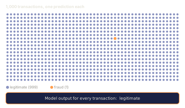
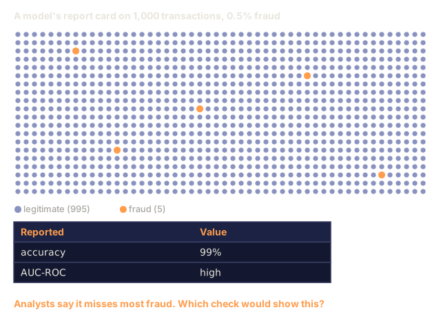
You build a fraud detection model. It hits 99.9% accuracy. You're ready to ship it, until you notice it predicts "not fraud" for every single transaction, no exceptions.
That's not a bug. It's the rational move when only 0.1% of transactions are fraudulent: guessing the majority class every time minimizes overall error. The model is technically correct and completely useless.
That pattern has a name: class imbalance, when the classes in a dataset are skewed badly enough that a model can win on the wrong metric just by favoring the majority class and ignoring the rest. It shows up everywhere classification actually matters. Disease diagnosis: 1% positive rate. Network intrusion: 0.01% attacks. Manufacturing defects: 0.5% defective. Spam filtering: 20% spam. Churn prediction: 5% churners. The more consequential the minority class, the rarer it tends to be.
Accuracy fails here because it treats every correct prediction as equal. Correctly labeling a legitimate transaction and correctly catching fraud both count as one point toward the same score, but catching fraud is the entire reason the model exists. What you actually need are metrics, techniques, and training strategies that force the model to notice the rare class it keeps ignoring.
The Concept
Why Accuracy Fails
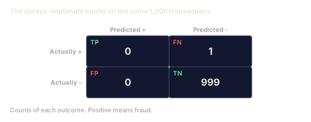
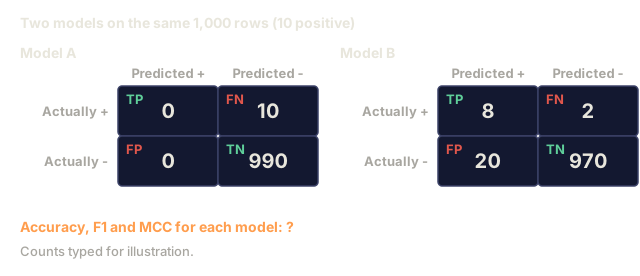
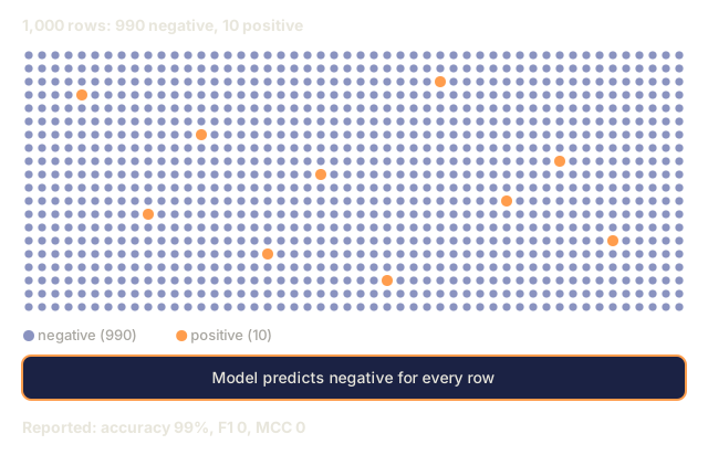
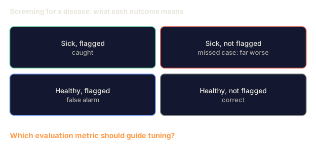
Take a dataset with 1000 samples: 990 negative, 10 positive. A model that always predicts negative produces this confusion matrix:
| Predicted Positive | Predicted Negative | |
|---|---|---|
| Actually Positive | 0 (TP) | 10 (FN) |
| Actually Negative | 0 (FP) | 990 (TN) |
Accuracy = (0 + 990) / 1000 = 99.0%
The model catches zero fraud. Zero disease. Zero defects. Accuracy still reports 99%. That's why accuracy is the wrong tool for imbalanced problems.
Better Metrics
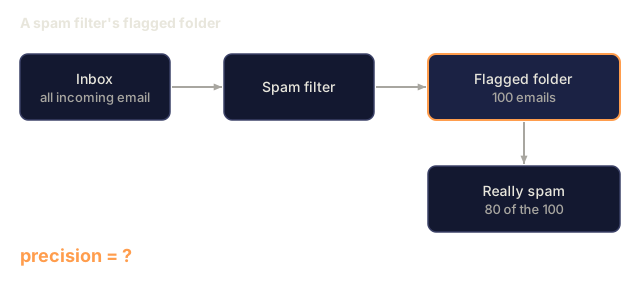
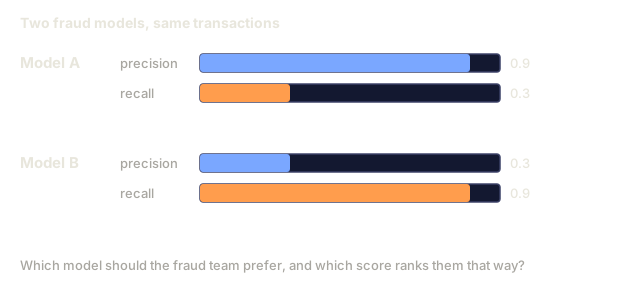
Precision = TP / (TP + FP). Of everything flagged as positive, how many actually are? High precision means few false alarms.
Recall = TP / (TP + FN). Of everything actually positive, how many did the model catch? High recall means few missed positives.
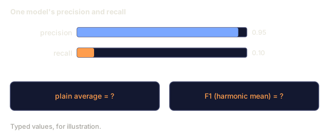
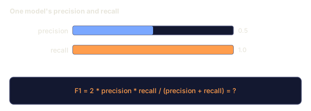
F1 Score = 2 * precision * recall / (precision + recall). The harmonic mean of the two. It punishes a big gap between precision and recall harder than a plain average would.
F-beta Score = (1 + beta^2) * precision * recall / (beta^2 * precision + recall). Set beta above 1 and recall matters more; set it below 1 and precision does. F2 shows up constantly in fraud detection, because missing fraud costs more than a false alarm.
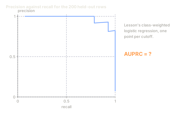
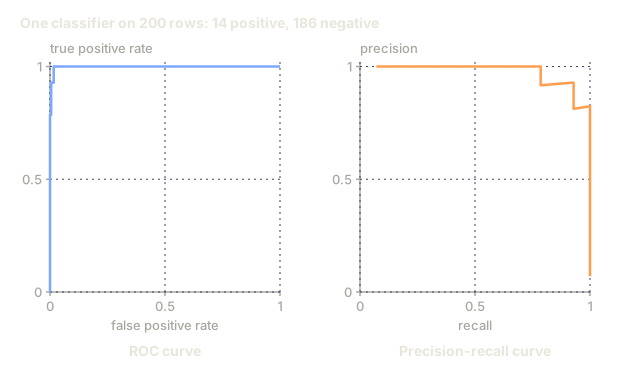
AUPRC (Area Under Precision-Recall Curve). Like AUC-ROC, but far more informative for imbalanced data: a random classifier scores an AUPRC equal to the positive class rate, not 0.5 like ROC, so real improvements actually show up in the number.
Matthews Correlation Coefficient = (TP * TN - FP * FN) / sqrt((TP+FP)(TP+FN)(TN+FP)(TN+FN)). Ranges from -1 to +1 and only climbs when the model does well on both classes, staying balanced even when the classes are wildly different sizes.
Run the "always predict negative" model through all of this: precision = 0/0 (undefined, usually set to 0), recall = 0/10 = 0, F1 = 0, MCC = 0. Every one of these correctly calls the model worthless.
The Imbalanced Data Pipeline

SMOTE: Synthetic Minority Oversampling Technique
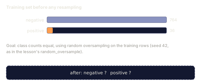
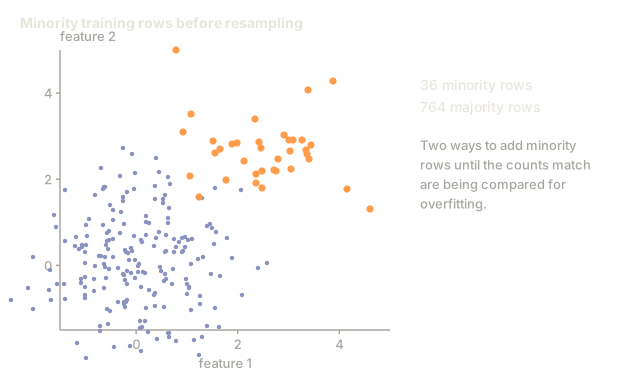
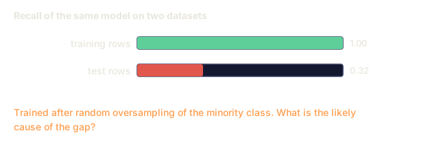
Random oversampling duplicates existing minority samples. That works, but it risks overfitting because the model keeps seeing identical points over and over.
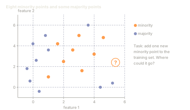
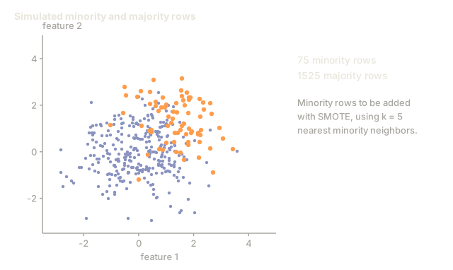
SMOTE creates new synthetic minority samples that are plausible but not copies. The algorithm:
- For each minority sample x, find its k nearest neighbors among other minority samples
- Pick one neighbor at random
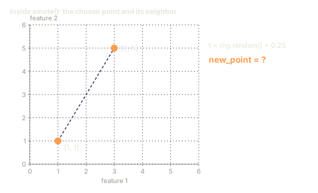
- Create a new sample on the line segment between x and that neighbor
The formula: new_sample = x + random(0, 1) * (neighbor - x)
It interpolates between real minority points, generating samples in the same region of feature space without copying anything that already exists.

Sampling Strategies Compared
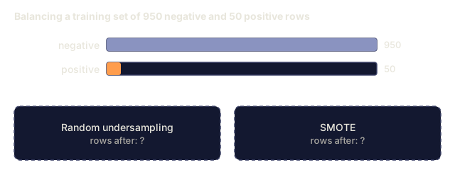
Random Oversampling: duplicate minority samples to match majority count.
- Pros: simple, no information loss
- Cons: exact duplicates cause overfitting, increases training time
Random Undersampling: remove majority samples to match minority count.
- Pros: fast training, simple
- Cons: throws away potentially useful majority data, higher variance
SMOTE: create synthetic minority samples via interpolation.
- Pros: generates new data points, reduces overfitting compared to random oversampling
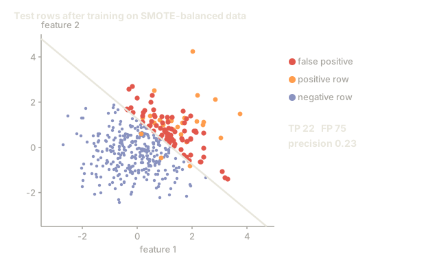
- Cons: can create noisy samples near the decision boundary, does not account for majority class distribution
| Strategy | Data Changed | Risk | When to Use |
|---|---|---|---|
| Oversample | Minority duplicated | Overfitting | Small datasets, moderate imbalance |
| Undersample | Majority removed | Information loss | Large datasets, want fast training |
| SMOTE | Synthetic minority added | Boundary noise | Moderate imbalance, enough minority samples for k-NN |
Class Weights
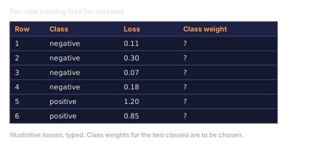
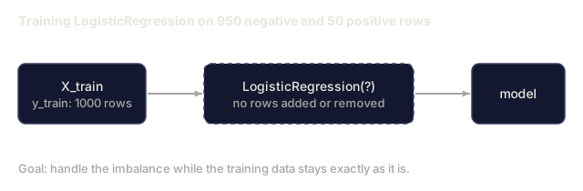
Instead of changing the data, change how the model treats errors: assign a higher weight to misclassifying the minority class.
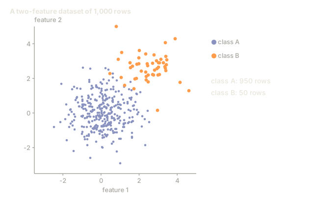
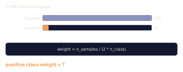
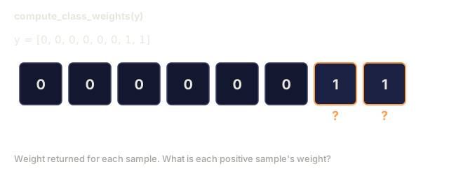
For a binary problem with 950 negative and 50 positive samples:
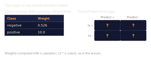
- Weight for negative class = n_samples / (2 * n_negative) = 1000 / (2 * 950) = 0.526
- Weight for positive class = n_samples / (2 * n_positive) = 1000 / (2 * 50) = 10.0
The positive class gets 19x the weight. Misclassifying one positive sample now costs as much as misclassifying 19 negative samples, so the model has no choice but to pay attention to the minority class.
In logistic regression, this modifies the loss function:
weighted_loss = -sum(w_i * [y_i * log(p_i) + (1-y_i) * log(1-p_i)])
where w_i depends on the class of sample i.
Class weights are mathematically equivalent to oversampling in expectation, but without creating new data points. That makes them faster and sidesteps the overfitting risk of duplicated samples.
Threshold Tuning
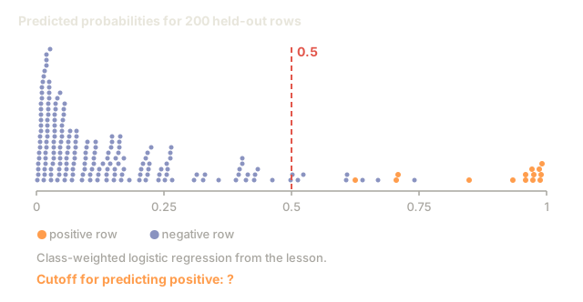
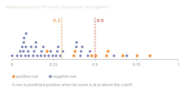
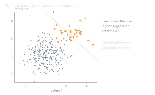
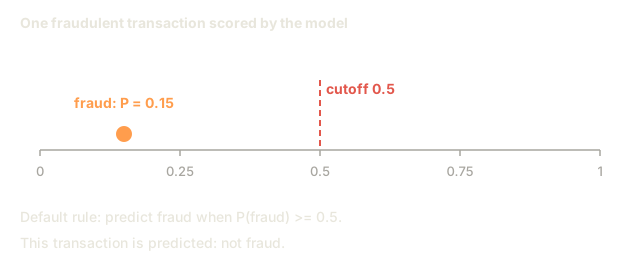
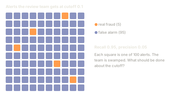
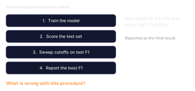
Most classifiers output a probability, and the default threshold is 0.5: if P(positive) >= 0.5, predict positive. But 0.5 is arbitrary, and when classes are imbalanced the optimal threshold is usually much lower. Threshold tuning means picking that cutoff on purpose: sweep candidate values, score each one on the metric you actually care about, and keep whichever threshold wins, instead of defaulting to 0.5 out of habit.
The process:
- Train a model
- Get predicted probabilities on the validation set
- Sweep thresholds from 0.0 to 1.0
- Compute F1 (or your chosen metric) at each threshold
- Pick the threshold that maximizes your metric

A model might output P(fraud) = 0.15 for a fraudulent transaction. At threshold 0.5, that gets classified as not fraud. At threshold 0.10, it's caught correctly. The probability calibration matters less than the ranking: as long as fraud scores higher than non-fraud, some threshold exists that separates them.
Cost-Sensitive Learning
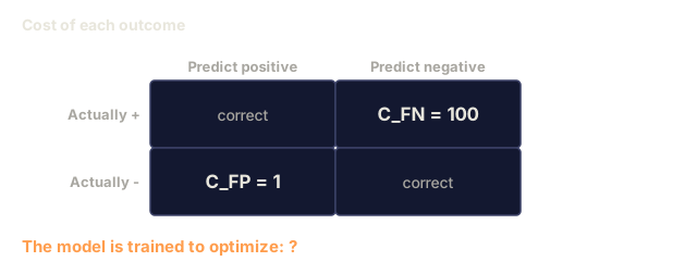
Cost-sensitive learning generalizes class weights. Instead of uniform costs, it assigns specific misclassification costs:
| Predict Positive | Predict Negative | |
|---|---|---|
| Actually Positive | 0 (correct) | C_FN = 100 |
| Actually Negative | C_FP = 1 | 0 (correct) |
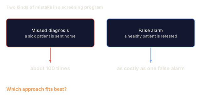
Missing a fraudulent transaction (FN) costs 100x more than a false alarm (FP), and the model optimizes for total cost, not total error count.
This is the most principled approach when you can actually estimate real-world costs. A missed cancer diagnosis costs something very different from a false alarm that leads to an extra biopsy. Making those costs explicit is what forces the right tradeoff.
Decision Flowchart

Build It
Step 1: Generate an imbalanced dataset
import numpy as np


def make_imbalanced_data(n_majority=950, n_minority=50, seed=42):
    rng = np.random.RandomState(seed)

    X_maj = rng.randn(n_majority, 2) * 1.0 + np.array([0.0, 0.0])
    X_min = rng.randn(n_minority, 2) * 0.8 + np.array([2.5, 2.5])

    X = np.vstack([X_maj, X_min])
    y = np.concatenate([np.zeros(n_majority), np.ones(n_minority)])

    shuffle_idx = rng.permutation(len(y))
    return X[shuffle_idx], y[shuffle_idx]
Step 2: SMOTE from scratch
def euclidean_distance(a, b):
    return np.sqrt(np.sum((a - b) ** 2))


def find_k_neighbors(X, idx, k):
    distances = []
    for i in range(len(X)):
        if i == idx:
            continue
        d = euclidean_distance(X[idx], X[i])
        distances.append((i, d))
    distances.sort(key=lambda x: x[1])
    return [d[0] for d in distances[:k]]


def smote(X_minority, k=5, n_synthetic=100, seed=42):
    rng = np.random.RandomState(seed)
    n_samples = len(X_minority)
    k = min(k, n_samples - 1)
    synthetic = []

    for _ in range(n_synthetic):
        idx = rng.randint(0, n_samples)
        neighbors = find_k_neighbors(X_minority, idx, k)
        neighbor_idx = neighbors[rng.randint(0, len(neighbors))]
        t = rng.random()
        new_point = X_minority[idx] + t * (X_minority[neighbor_idx] - X_minority[idx])
        synthetic.append(new_point)

    return np.array(synthetic)
Step 3: Random oversampling and undersampling
def random_oversample(X, y, seed=42):
    rng = np.random.RandomState(seed)
    classes, counts = np.unique(y, return_counts=True)
    max_count = counts.max()

    X_resampled = list(X)
    y_resampled = list(y)

    for cls, count in zip(classes, counts):
        if count < max_count:
            cls_indices = np.where(y == cls)[0]
            n_needed = max_count - count
            chosen = rng.choice(cls_indices, size=n_needed, replace=True)
            X_resampled.extend(X[chosen])
            y_resampled.extend(y[chosen])

    X_out = np.array(X_resampled)
    y_out = np.array(y_resampled)
    shuffle = rng.permutation(len(y_out))
    return X_out[shuffle], y_out[shuffle]


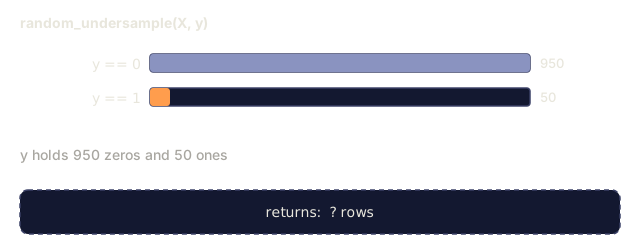
def random_undersample(X, y, seed=42):
    rng = np.random.RandomState(seed)
    classes, counts = np.unique(y, return_counts=True)
    min_count = counts.min()

    X_resampled = []
    y_resampled = []

    for cls in classes:
        cls_indices = np.where(y == cls)[0]
        chosen = rng.choice(cls_indices, size=min_count, replace=False)
        X_resampled.extend(X[chosen])
        y_resampled.extend(y[chosen])

    X_out = np.array(X_resampled)
    y_out = np.array(y_resampled)
    shuffle = rng.permutation(len(y_out))
    return X_out[shuffle], y_out[shuffle]
Step 4: Logistic regression with class weights
def sigmoid(z):
    return 1.0 / (1.0 + np.exp(-np.clip(z, -500, 500)))


def logistic_regression_weighted(X, y, weights, lr=0.01, epochs=200):
    n_samples, n_features = X.shape
    w = np.zeros(n_features)
    b = 0.0

    for _ in range(epochs):
        z = X @ w + b
        pred = sigmoid(z)
        error = pred - y
        weighted_error = error * weights

        gradient_w = (X.T @ weighted_error) / n_samples
        gradient_b = np.mean(weighted_error)

        w -= lr * gradient_w
        b -= lr * gradient_b

    return w, b


def compute_class_weights(y):
    classes, counts = np.unique(y, return_counts=True)
    n_samples = len(y)
    n_classes = len(classes)
    weight_map = {}
    for cls, count in zip(classes, counts):
        weight_map[cls] = n_samples / (n_classes * count)
    return np.array([weight_map[yi] for yi in y])
Step 5: Threshold tuning
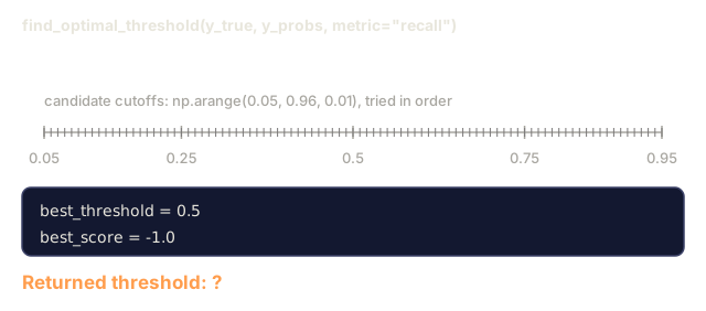
def find_optimal_threshold(y_true, y_probs, metric="f1"):
    best_threshold = 0.5
    best_score = -1.0

    for threshold in np.arange(0.05, 0.96, 0.01):
        y_pred = (y_probs >= threshold).astype(int)
        tp = np.sum((y_pred == 1) & (y_true == 1))
        fp = np.sum((y_pred == 1) & (y_true == 0))
        fn = np.sum((y_pred == 0) & (y_true == 1))

        if metric == "f1":
            precision = tp / (tp + fp) if (tp + fp) > 0 else 0.0
            recall = tp / (tp + fn) if (tp + fn) > 0 else 0.0
            score = 2 * precision * recall / (precision + recall) if (precision + recall) > 0 else 0.0
        elif metric == "recall":
            score = tp / (tp + fn) if (tp + fn) > 0 else 0.0
        elif metric == "precision":
            score = tp / (tp + fp) if (tp + fp) > 0 else 0.0

        if score > best_score:
            best_score = score
            best_threshold = threshold

    return best_threshold, best_score
Step 6: Evaluation functions
def confusion_matrix_values(y_true, y_pred):
    tp = np.sum((y_pred == 1) & (y_true == 1))
    tn = np.sum((y_pred == 0) & (y_true == 0))
    fp = np.sum((y_pred == 1) & (y_true == 0))
    fn = np.sum((y_pred == 0) & (y_true == 1))
    return tp, tn, fp, fn


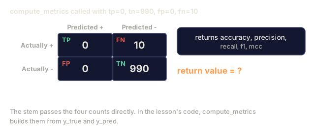
def compute_metrics(y_true, y_pred):
    tp, tn, fp, fn = confusion_matrix_values(y_true, y_pred)
    accuracy = (tp + tn) / (tp + tn + fp + fn)
    precision = tp / (tp + fp) if (tp + fp) > 0 else 0.0
    recall = tp / (tp + fn) if (tp + fn) > 0 else 0.0
    f1 = 2 * precision * recall / (precision + recall) if (precision + recall) > 0 else 0.0

    denom = np.sqrt(float((tp + fp) * (tp + fn) * (tn + fp) * (tn + fn)))
    mcc = (tp * tn - fp * fn) / denom if denom > 0 else 0.0

    return {
        "accuracy": accuracy,
        "precision": precision,
        "recall": recall,
        "f1": f1,
        "mcc": mcc,
    }
Step 7: Compare all approaches
X, y = make_imbalanced_data(950, 50, seed=42)
split = int(0.8 * len(y))
X_train, X_test = X[:split], X[split:]
y_train, y_test = y[:split], y[split:]

# Baseline: no treatment
w_base, b_base = logistic_regression_weighted(
    X_train, y_train, np.ones(len(y_train)), lr=0.1, epochs=300
)
probs_base = sigmoid(X_test @ w_base + b_base)
preds_base = (probs_base >= 0.5).astype(int)

# Oversampled
X_over, y_over = random_oversample(X_train, y_train)
w_over, b_over = logistic_regression_weighted(
    X_over, y_over, np.ones(len(y_over)), lr=0.1, epochs=300
)
preds_over = (sigmoid(X_test @ w_over + b_over) >= 0.5).astype(int)

# SMOTE
minority_mask = y_train == 1
X_minority = X_train[minority_mask]
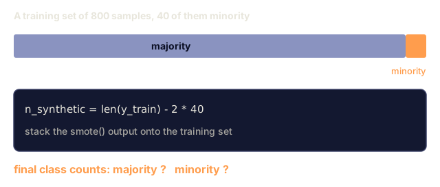
synthetic = smote(X_minority, k=5, n_synthetic=len(y_train) - 2 * int(minority_mask.sum()))
X_smote = np.vstack([X_train, synthetic])
y_smote = np.concatenate([y_train, np.ones(len(synthetic))])
w_sm, b_sm = logistic_regression_weighted(
    X_smote, y_smote, np.ones(len(y_smote)), lr=0.1, epochs=300
)
preds_smote = (sigmoid(X_test @ w_sm + b_sm) >= 0.5).astype(int)

# Class weights
sample_weights = compute_class_weights(y_train)
w_cw, b_cw = logistic_regression_weighted(
    X_train, y_train, sample_weights, lr=0.1, epochs=300
)
probs_cw = sigmoid(X_test @ w_cw + b_cw)
preds_cw = (probs_cw >= 0.5).astype(int)

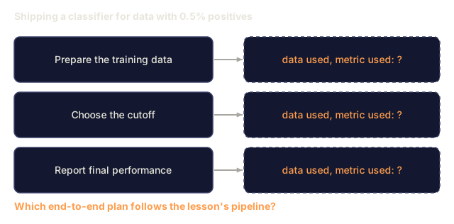
# Threshold tuning (tune on held-out validation set, not test set)
val_split = int(0.75 * len(y_train))
X_tr, X_val = X_train[:val_split], X_train[val_split:]
y_tr, y_val = y_train[:val_split], y_train[val_split:]
val_weights = compute_class_weights(y_tr)
w_val, b_val = logistic_regression_weighted(X_tr, y_tr, val_weights, lr=0.1, epochs=300)
probs_val = sigmoid(X_val @ w_val + b_val)
best_thresh, best_f1 = find_optimal_threshold(y_val, probs_val, metric="f1")
preds_thresh = (probs_cw >= best_thresh).astype(int)
The code file runs all of this in a single script and prints results.
Use It
With scikit-learn and imbalanced-learn, these techniques are one-liners:
from sklearn.linear_model import LogisticRegression
from sklearn.metrics import classification_report, f1_score
from sklearn.model_selection import train_test_split
from imblearn.over_sampling import SMOTE
from imblearn.under_sampling import RandomUnderSampler
from imblearn.pipeline import Pipeline

X_train, X_test, y_train, y_test = train_test_split(X, y, stratify=y)

model_weighted = LogisticRegression(class_weight="balanced")
model_weighted.fit(X_train, y_train)
print(classification_report(y_test, model_weighted.predict(X_test)))

smote = SMOTE(random_state=42)
X_resampled, y_resampled = smote.fit_resample(X_train, y_train)
model_smote = LogisticRegression()
model_smote.fit(X_resampled, y_resampled)
print(classification_report(y_test, model_smote.predict(X_test)))

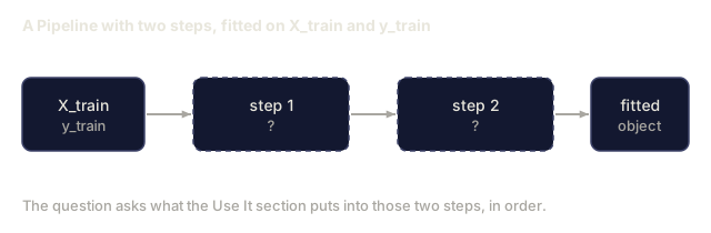
pipeline = Pipeline([
    ("smote", SMOTE()),
    ("model", LogisticRegression(class_weight="balanced")),
])
pipeline.fit(X_train, y_train)
print(classification_report(y_test, pipeline.predict(X_test)))
The from-scratch implementations show exactly what each technique does. SMOTE is just k-NN interpolation on the minority class. Class weights multiply the loss. Threshold tuning is a for-loop over cutoffs. No magic.
Ship It
This lesson produces:
outputs/skill-imbalanced-data.md, a decision checklist for handling imbalanced classification problems
Exercises
-
Borderline-SMOTE: modify the SMOTE implementation to only generate synthetic samples for minority points that are near the decision boundary (those whose k-nearest neighbors include majority class samples). Compare results with standard SMOTE on a dataset where classes overlap.
-
Cost matrix optimization: implement cost-sensitive learning where the cost matrix is a parameter. Create a function that takes a cost matrix and returns optimal predictions that minimize expected cost. Test with different cost ratios (1:10, 1:100, 1:1000) and plot how the precision-recall tradeoff changes.
-
Threshold calibration: implement Platt scaling (fit a logistic regression on the model's raw outputs to produce calibrated probabilities). Compare the precision-recall curve before and after calibration. Show that calibration does not change the ranking (AUC stays the same) but makes the probabilities more meaningful.
-
Ensemble with balanced bagging: train multiple models, each on a balanced bootstrap sample (all minority + random subset of majority). Average their predictions. Compare this approach against a single model with SMOTE. Measure both performance and variance across runs.
-
Imbalance ratio experiment: take a balanced dataset and progressively increase the imbalance ratio (50/50, 70/30, 90/10, 95/5, 99/1). For each ratio, train with and without SMOTE. Plot F1 vs imbalance ratio for both approaches. At what ratio does SMOTE start making a meaningful difference?
Key Terms
| Term | What people say | What it actually means |
|---|---|---|
| Class imbalance | "One class has way more samples" | The distribution of classes in the dataset is significantly skewed, causing models to favor the majority class |
| SMOTE | "Synthetic oversampling" | Creates new minority samples by interpolating between existing minority samples and their k-nearest minority neighbors |
| Class weights | "Making errors on rare classes more expensive" | Multiplying the loss function by class-specific weights so the model penalizes minority misclassification more heavily |
| Threshold tuning | "Moving the decision boundary" | Changing the probability cutoff for classification from the default 0.5 to a value that optimizes the desired metric |
| Precision-recall tradeoff | "You cannot have both" | Lowering the threshold catches more positives (higher recall) but also flags more false positives (lower precision), and vice versa |
| AUPRC | "Area under the PR curve" | Summarizes the precision-recall curve into a single number; more informative than AUC-ROC when classes are heavily imbalanced |
| Matthews Correlation Coefficient | "The balanced metric" | A correlation between predicted and actual labels that produces a high score only when the model performs well on both classes |
| Cost-sensitive learning | "Different mistakes cost different amounts" | Incorporating real-world misclassification costs into the training objective so the model optimizes for total cost, not error count |
| Random oversampling | "Duplicate the minority" | Repeating minority class samples to balance class counts; simple but risks overfitting to duplicated points |
Further Reading
- SMOTE: Synthetic Minority Over-sampling Technique (Chawla et al., 2002) — the original SMOTE paper, still the most cited work on imbalanced learning
- Learning from Imbalanced Data (He & Garcia, 2009) — comprehensive survey covering sampling, cost-sensitive, and algorithmic approaches
- imbalanced-learn documentation — Python library with SMOTE variants, undersampling strategies, and pipeline integration
- The Precision-Recall Plot Is More Informative than the ROC Plot (Saito & Rehmsmeier, 2015) — when and why to prefer PR curves over ROC curves for imbalanced problems
Code
- imbalanced.py (python, 353 lines)