Norms and Distances
Your distance function decides what "similar" means. Pick the wrong one and everything built on top of it breaks.
Learning Objectives
- Implement L1, L2, cosine, Mahalanobis, Jaccard, and edit distance functions from scratch
- Select the appropriate distance metric for a given ML task and explain why alternatives fail
- Connect L1 and L2 norms to LASSO and Ridge regularization and their geometric constraint regions
- Demonstrate how the same dataset produces different nearest neighbors under different metrics
The Problem
You have two vectors. Maybe they're word embeddings, maybe user profiles, maybe raw pixel arrays. The question is always the same: how close are they?
The answer depends entirely on which distance function you pick. Two points can be nearest neighbors under one metric and sit far apart under another, and that choice cascades into everything downstream: your KNN classifier, your recommendation engine, your vector database, your clustering algorithm, your loss function. Get it wrong and the model ends up optimizing for the wrong notion of similarity.
There's no universal best distance. L2 works for spatial data. Cosine similarity dominates NLP. Jaccard handles sets. Edit distance handles strings. Mahalanobis accounts for correlations. Wasserstein moves probability mass. Each one encodes a different assumption about what "similar" means.
This lesson builds every major distance function from scratch, shows you when each one is the right tool, and demonstrates how the same data produces different nearest neighbors depending on which metric you use.
The Concept
Norms: measuring vector magnitude
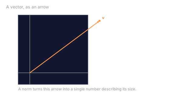
A norm measures the "size" of a vector. Every distance function between two vectors is just the norm of their difference: d(a, b) = ||a - b||. Learn the norms, and you already understand the distances.
L1 Norm (Manhattan distance)
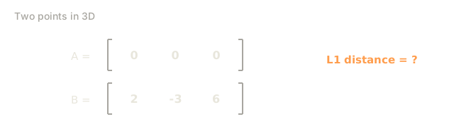
The L1 norm sums the absolute values of all components.
||x||_1 = |x_1| + |x_2| + ... + |x_n|
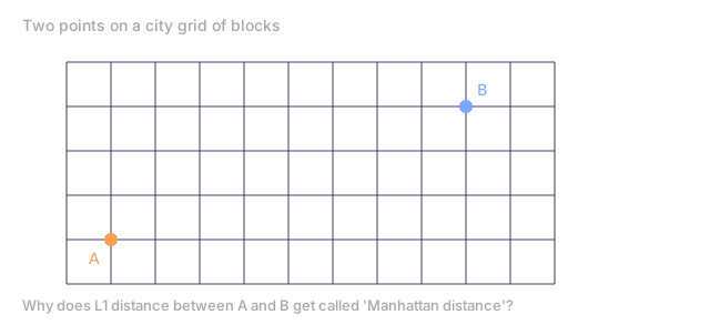
Manhattan distance is the same thing under a friendlier name: it's how far you'd walk on a city grid where you can only move along axes, no diagonals allowed.
Point A = (1, 1)
Point B = (4, 5)

L1 distance = |4-1| + |5-1| = 3 + 4 = 7

On a grid, you walk 3 blocks east and 4 blocks north.
When to use L1:
- High-dimensional sparse data (text features, one-hot encodings)
- When you want robustness to outliers, since one huge difference doesn't dominate the sum
- Feature selection problems, where L1 regularization promotes sparsity
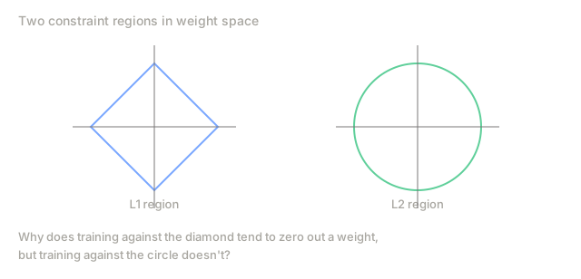
Connection to L1 regularization (Lasso): adding ||w||_1 to your loss function penalizes the sum of absolute weight values. That pushes small weights to exactly zero, which is automatic feature selection. The penalty carves out diamond-shaped constraint regions in weight space, and the diamond's corners sit on the axes, exactly where some weights hit zero.
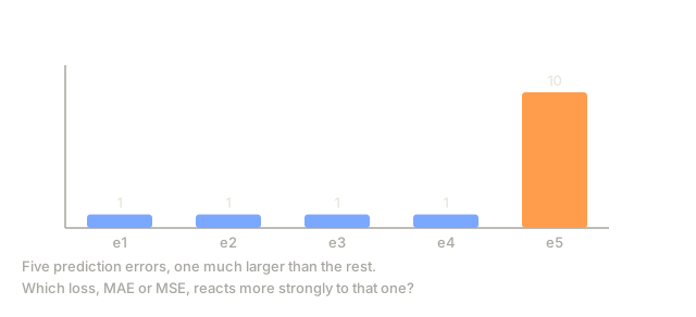
Connection to loss functions: Mean Absolute Error (MAE) is just the average L1 distance between predictions and targets. It penalizes every error linearly, which makes it more robust to outliers than MSE.
L2 Norm (Euclidean distance)
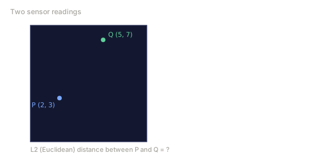
The L2 norm is the straight-line distance: the square root of the sum of squared components.
||x||_2 = sqrt(x_1^2 + x_2^2 + ... + x_n^2)
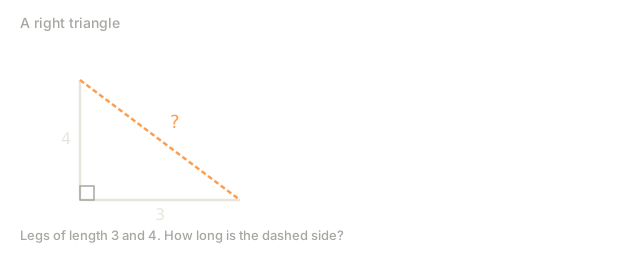
It's the distance from geometry class, Pythagoras extended to n dimensions.
Point A = (1, 1)
Point B = (4, 5)

L2 distance = sqrt((4-1)^2 + (5-1)^2) = sqrt(9 + 16) = sqrt(25) = 5.0

The straight line, cutting diagonally through the grid.
When to use L2:
- Low-to-medium dimensional continuous data
- When the feature scales are comparable
- Physical distances (spatial data, sensor readings)
- Image similarity at the pixel level
Connection to L2 regularization (Ridge): adding ||w||_2^2 to your loss function penalizes large weights. Unlike L1, it doesn't push weights to zero; it shrinks all of them toward zero proportionally. The penalty carves out circular constraint regions with no corners on the axes, so weights get small but rarely land on exactly zero.
Connection to loss functions: Mean Squared Error (MSE) is the average of squared L2 distances. Squaring means large errors get punished far more than small ones.
MAE (L1 loss):  |y - y_hat|         Linear penalty. Robust to outliers.
MSE (L2 loss):  (y - y_hat)^2       Quadratic penalty. Sensitive to outliers.
Lp Norms: the general family
L1 and L2 are both special cases of one general formula, the Lp norm:
||x||_p = (|x_1|^p + |x_2|^p + ... + |x_n|^p)^(1/p)
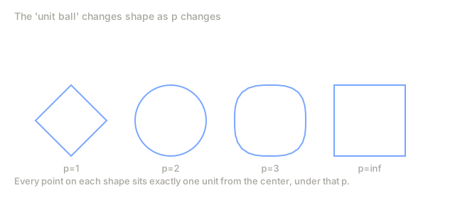
Change p and you change the shape of the "unit ball" (the set of every point sitting at distance 1 from the origin):
p=1:    Diamond shape      (corners on axes)
p=2:    Circle/sphere      (the usual round ball)
p=3:    Superellipse       (rounded square)
p=inf:  Square/hypercube   (flat sides along axes)
L-infinity Norm (Chebyshev distance)
Push p to infinity and the Lp norm collapses to a single number: the maximum absolute component.
||x||_inf = max(|x_1|, |x_2|, ..., |x_n|)
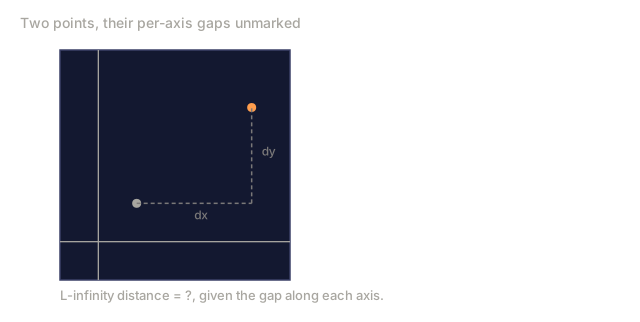
The distance between two points comes down to whichever single dimension differs the most; every other dimension gets ignored entirely.
Point A = (1, 1)
Point B = (4, 5)

L-inf distance = max(|4-1|, |5-1|) = max(3, 4) = 4
When to use L-infinity:
- When the worst-case deviation in any single dimension matters
- Game boards (a king in chess moves in L-infinity: one step in any direction costs 1)
- Manufacturing tolerances (every dimension must be within spec)
Cosine Similarity and Cosine Distance
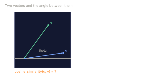
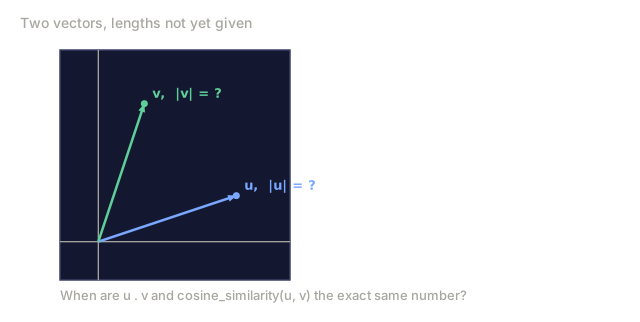
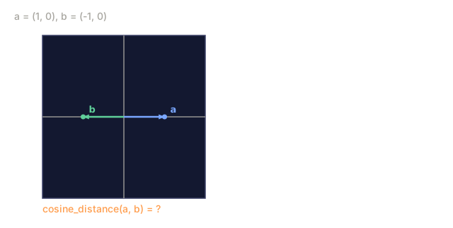
Cosine similarity measures the angle between two vectors and ignores their magnitude entirely.
cos_sim(a, b) = (a . b) / (||a||_2 * ||b||_2)
It ranges from -1 (opposite directions) to +1 (same direction), with perpendicular vectors sitting at exactly 0.
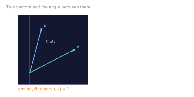
Cosine distance is the same idea flipped into a distance: cosine_distance = 1 - cosine_similarity, ranging from 0 (identical direction) to 2 (opposite direction).
a = (1, 0)    b = (1, 1)

cos_sim = (1*1 + 0*1) / (1 * sqrt(2)) = 1/sqrt(2) = 0.707
cos_dist = 1 - 0.707 = 0.293
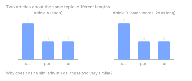
Why cosine dominates NLP and embeddings: document length shouldn't affect similarity. A document about cats that runs twice as long as another cat document should still count as similar, and cosine similarity delivers that because it only cares about direction, not length. Two documents with the same word distribution but different lengths point in the same direction and score a perfect 1.0.
When to use cosine similarity:
- Text similarity (TF-IDF vectors, word embeddings, sentence embeddings)
- Any domain where magnitude is noise and direction is signal
- Recommendation systems (user preference vectors)
- Embedding search (vector databases almost always use cosine or dot product)
Dot Product Similarity vs Cosine Similarity
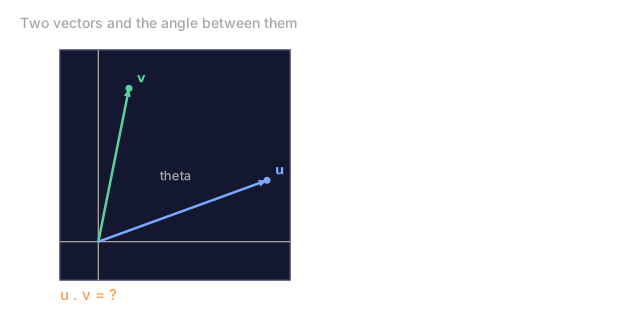
The dot product of two vectors is:
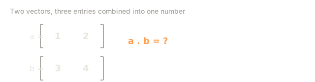
a . b = a_1*b_1 + a_2*b_2 + ... + a_n*b_n
      = ||a|| * ||b|| * cos(angle)
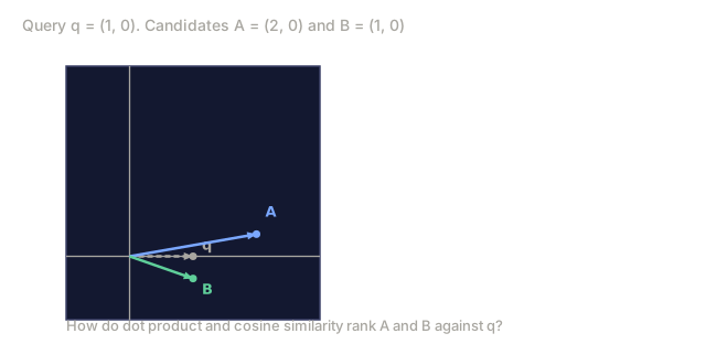
Cosine similarity is just the dot product normalized by both magnitudes, so once both vectors are unit-normalized (magnitude 1), the two measures collapse into the same number.
If ||a|| = 1 and ||b|| = 1:
    a . b = cos(angle between a and b)
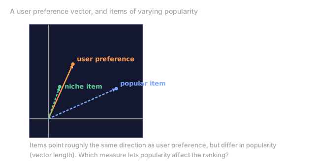
Where they diverge: the raw dot product still carries magnitude information, so a vector with a larger magnitude scores higher. Some retrieval systems want exactly that, letting magnitude act as an implicit popularity or importance signal so "popular" items rank higher.
a = (3, 0)    b = (1, 0)    c = (0, 1)

dot(a, b) = 3     dot(a, c) = 0
cos(a, b) = 1.0   cos(a, c) = 0.0

Both agree on direction, but dot product also reflects magnitude.
In practice:
- Use cosine similarity when you want pure directional similarity
- Use dot product when magnitudes carry meaningful information
- Many vector databases (Pinecone, Weaviate, Qdrant) let you choose between them
- If your embeddings are L2-normalized, the choice doesn't matter
Mahalanobis Distance
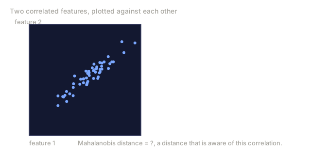
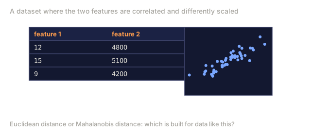
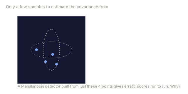
Mahalanobis distance accounts for the covariance structure of the data, which matters because plain Euclidean distance treats every dimension as equally important even when your features are correlated or sit on different scales.
d_M(x, y) = sqrt((x - y)^T * S^(-1) * (x - y))
where S is the covariance matrix of the data: a square matrix whose diagonal holds each feature's variance and whose off-diagonal entries capture how much pairs of features vary together.
Intuitively: Mahalanobis distance first decorrelates and normalizes the data (whitening), then computes L2 distance in that transformed space. If S is the identity matrix (uncorrelated, unit variance features), Mahalanobis distance reduces to Euclidean distance.
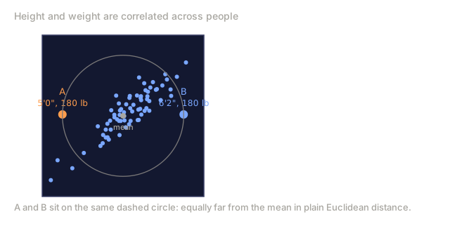
Example: height and weight are correlated.
Someone 6'2" and 180 lbs is not unusual.
Someone 5'0" and 180 lbs is unusual.

Euclidean distance might say they are equally far from the mean.
Mahalanobis distance correctly identifies the second as an outlier
because it accounts for the height-weight correlation.
When to use Mahalanobis distance:
- Outlier detection (points with large Mahalanobis distance from the mean are outliers)
- Classification when features have different scales and correlations
- When you have enough data to estimate a reliable covariance matrix
- Quality control in manufacturing (multivariate process monitoring)
Jaccard Similarity (for sets)
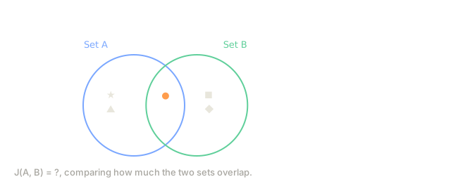
Jaccard similarity measures how much two sets overlap.
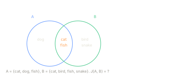
J(A, B) = |A intersect B| / |A union B|
It ranges from 0 (no overlap) to 1 (identical sets), and Jaccard distance is just 1 minus that.
A = {cat, dog, fish}
B = {cat, bird, fish, snake}

Intersection = {cat, fish}         size = 2
Union = {cat, dog, fish, bird, snake}  size = 5

Jaccard similarity = 2/5 = 0.4
Jaccard distance = 0.6
When to use Jaccard:
- Comparing sets of tags, categories, or features
- Document similarity based on word presence (not frequency)
- Near-duplicate detection (MinHash approximation of Jaccard)
- Comparing binary feature vectors (presence/absence data)
- Evaluating segmentation models (Intersection over Union = Jaccard)
Edit Distance (Levenshtein Distance)
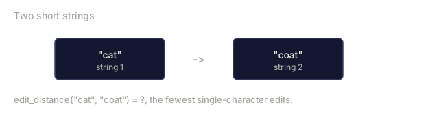
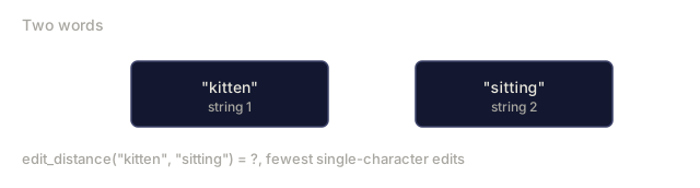
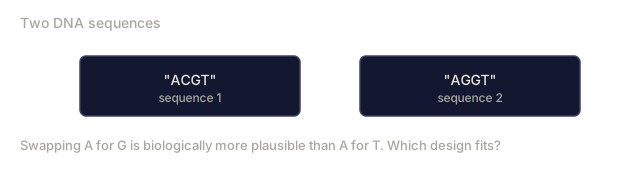
Edit distance counts the minimum number of single-character operations (insert, delete, or substitute) needed to turn one string into another.
"kitten" -> "sitting"

kitten -> sitten  (substitute k -> s)
sitten -> sittin  (substitute e -> i)
sittin -> sitting (insert g)

Edit distance = 3
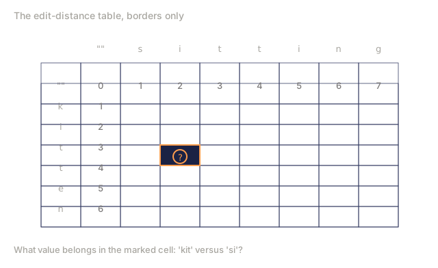
It's computed with dynamic programming: fill a matrix where entry (i, j) holds the edit distance between the first i characters of string A and the first j characters of string B.
        ""  s  i  t  t  i  n  g
    ""   0  1  2  3  4  5  6  7
    k    1  1  2  3  4  5  6  7
    i    2  2  1  2  3  4  5  6
    t    3  3  2  1  2  3  4  5
    t    4  4  3  2  1  2  3  4
    e    5  5  4  3  2  2  3  4
    n    6  6  5  4  3  3  2  3
When to use edit distance:
- Spell checking and correction
- DNA sequence alignment (with weighted operations)
- Fuzzy string matching
- Deduplication of messy text data
KL Divergence (not a distance, but used like one)
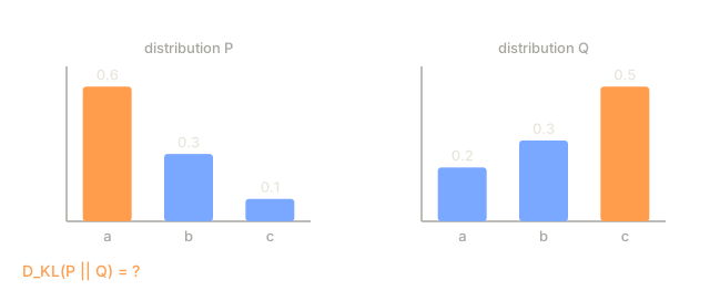
KL divergence measures how one probability distribution differs from another. It's covered properly in Lesson 09, but it earns a mention here because people casually call it a "distance" when it isn't one.
D_KL(P || Q) = sum(p(x) * log(p(x) / q(x)))
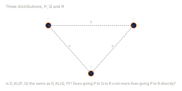
Critical property: KL divergence is not symmetric.
D_KL(P || Q) != D_KL(Q || P)
That alone disqualifies it as a distance metric, and it fails the triangle inequality too. It's a divergence, not a distance.
Forward KL (D_KL(P || Q)) is "mean-seeking": Q tries to cover all modes of P. Reverse KL (D_KL(Q || P)) is "mode-seeking": Q focuses on a single mode of P.
When you see KL divergence:
- VAEs (the KL term in the ELBO, the evidence lower bound, pushes the latent distribution toward a prior)
- Knowledge distillation (student tries to match teacher's distribution)
- RLHF (the KL penalty keeps the fine-tuned model close to the base model)
- Policy gradient methods (constraining policy updates)
Wasserstein Distance (Earth Mover's Distance)
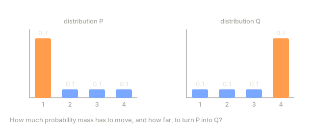
Wasserstein distance measures the minimum "work" needed to turn one probability distribution into another: if one distribution is a pile of dirt and the other a hole, how much dirt do you have to move, and how far?
W(P, Q) = inf over all transport plans gamma of E[d(x, y)]
For 1D distributions, it simplifies to the integral of the absolute difference of the cumulative distribution functions:
W_1(P, Q) = integral |CDF_P(x) - CDF_Q(x)| dx
Why Wasserstein matters:
- It's a true metric (symmetric, satisfies triangle inequality)
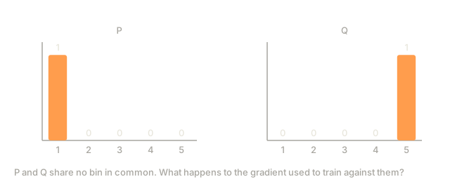
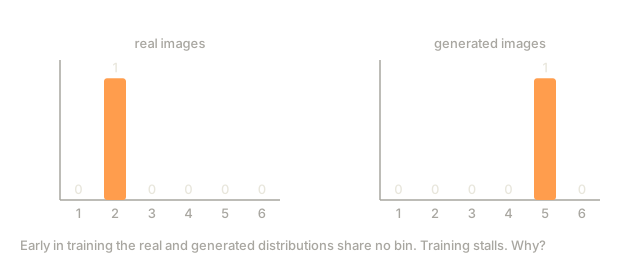
- It provides gradients even when distributions don't overlap, where KL divergence blows up to infinity
- That property made it central to Wasserstein GANs (WGANs), which fixed the training instability of the original GAN formulation
Distributions with no overlap:

P: [1, 0, 0, 0, 0]    Q: [0, 0, 0, 0, 1]

KL divergence: infinity (log of zero)
Wasserstein: 4 (move all mass 4 bins)

Wasserstein gives a meaningful gradient. KL does not.
When to use Wasserstein:
- GAN training (WGAN, WGAN-GP)
- Comparing distributions that may not overlap
- Optimal transport problems
- Image retrieval (comparing color histograms)
Why Different Tasks Need Different Distances
| Task | Best distance | Why |
|---|---|---|
| Text similarity | Cosine | Magnitude is noise, direction is meaning |
| Image pixel comparison | L2 | Spatial relationships matter, features are comparable scale |
| Sparse high-dim features | L1 | Robust, does not amplify rare large differences |
| Set overlap (tags, categories) | Jaccard | Data is naturally set-valued, not vectorial |
| String matching | Edit distance | Operations map to human editing intuition |
| Outlier detection | Mahalanobis | Accounts for feature correlations and scales |
| Comparing distributions | KL divergence | Measures information lost by using Q instead of P |
| GAN training | Wasserstein | Provides gradients even when distributions do not overlap |
| Embeddings (vector DB) | Cosine or dot product | Embeddings are trained to encode meaning in direction |
| Recommendation | Dot product | Magnitude can encode popularity or confidence |
| DNA sequences | Weighted edit distance | Substitution costs vary by nucleotide pair |
| Manufacturing QC | L-infinity | Worst-case deviation in any dimension matters |
Connection to Loss Functions
Loss functions are distance functions in disguise, applied to predictions versus targets.
Loss function       Distance it uses       Behavior
MSE                 L2 squared             Penalizes large errors heavily
MAE                 L1                     Penalizes all errors equally
Huber loss          L1 for large errors,   Best of both: robust to outliers,
                    L2 for small errors    smooth gradient near zero
Cross-entropy       KL divergence          Measures distribution mismatch
Hinge loss          max(0, margin - d)     Only penalizes below margin
Triplet loss        L2 (typically)         Pulls positives close, pushes
                                           negatives away
Contrastive loss    L2                     Similar pairs close, dissimilar
                                           pairs beyond margin
Connection to Regularization
Regularization works by adding a norm penalty on the weights to the loss function.
L1 regularization (Lasso):   loss + lambda * ||w||_1
  -> Sparse weights. Some weights become exactly zero.
  -> Automatic feature selection.
  -> Solution has corners (non-differentiable at zero).

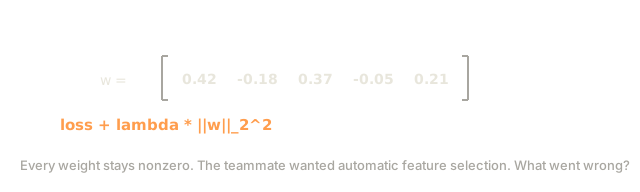
L2 regularization (Ridge):   loss + lambda * ||w||_2^2
  -> Small weights. All weights shrink toward zero.
  -> No feature selection (nothing goes to exactly zero).
  -> Smooth solution everywhere.

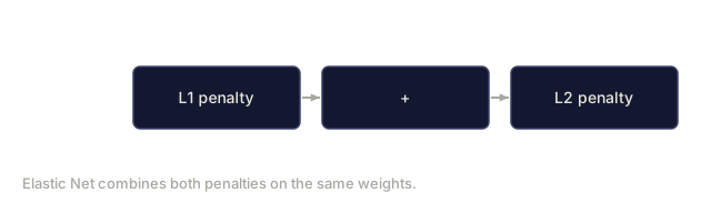
Elastic Net:                  loss + lambda_1 * ||w||_1 + lambda_2 * ||w||_2^2
  -> Combines sparsity of L1 with stability of L2.
  -> Groups of correlated features are kept or dropped together.
Why L1 produces sparsity and L2 doesn't: picture the constraint region in 2D weight space. L1 draws a diamond, L2 draws a circle. The loss function's elliptical contours are most likely to first touch the diamond at one of its corners, where a weight lands on exactly zero. Against the circle, they touch at a smooth point instead, where both weights stay nonzero.
Nearest Neighbor Search
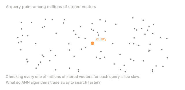
Every distance function implies a nearest neighbor search problem: given a query point, find the closest points in a dataset.
Exact nearest neighbor search costs O(n * d) per query across n points in d dimensions, and at real dataset sizes that's too slow to run online.
Approximate Nearest Neighbor (ANN) algorithms trade a small amount of accuracy for a massive speed gain:
Algorithm         Approach                      Used by
KD-trees          Axis-aligned space partition   scikit-learn (low-dim)
Ball trees        Nested hyperspheres            scikit-learn (medium-dim)
LSH               Random hash projections        Near-duplicate detection
HNSW              Hierarchical navigable         FAISS, Qdrant, Weaviate
                  small-world graph
IVF               Inverted file index with       FAISS (billion-scale)
                  cluster-based search
Product quant.    Compress vectors, search       FAISS (memory-constrained)
                  in compressed space
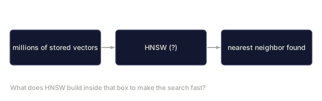
HNSW (Hierarchical Navigable Small World) is the dominant algorithm behind modern vector databases. It builds a multi-layer graph where each node connects to its approximate nearest neighbors, and a search starts at the sparse top layer for long jumps, then descends toward the dense bottom layer for short ones.




Build It
Step 1: All norm and distance functions
code/distances.py has the complete implementation. Every function is built from scratch with nothing but basic Python math, no NumPy shortcuts.
Step 2: Same data, different distances, different neighbors
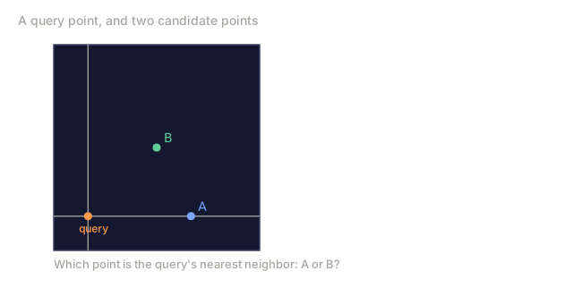
The demo in distances.py builds a dataset, picks a query point, and walks through how the nearest neighbor shifts depending on which metric you use. The point that's "closest" under L1 isn't necessarily closest under L2 or cosine.
Step 3: Embedding similarity search
The code also runs a mock embedding similarity search, finding the most similar "documents" to a query under cosine similarity versus L2 distance, and shows how the rankings diverge between the two.
Use It
The most common practical use of all this: finding similar items in a vector database.
import numpy as np

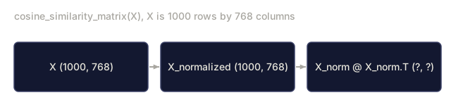
def cosine_similarity_matrix(X):
    norms = np.linalg.norm(X, axis=1, keepdims=True)
    norms = np.where(norms == 0, 1, norms)
    X_normalized = X / norms
    return X_normalized @ X_normalized.T

embeddings = np.random.randn(1000, 768)

sim_matrix = cosine_similarity_matrix(embeddings)

query_idx = 0
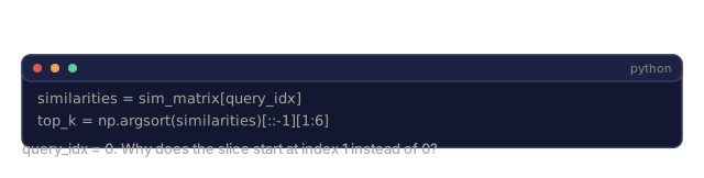
similarities = sim_matrix[query_idx]
top_k = np.argsort(similarities)[::-1][1:6]
print(f"Top 5 most similar to item 0: {top_k}")
print(f"Similarities: {similarities[top_k]}")
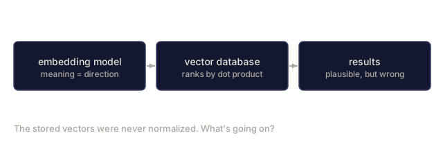
This is what actually happens when you call model.encode(text) and then search a vector database. The embedding model maps text to vectors, and the vector database computes cosine similarity (or dot product) between your query vector and every stored vector, leaning on ANN algorithms so it never has to check them all.
Ship It
This lesson produces:
outputs/prompt-distance-chooser.md, a prompt that walks you through picking the right distance metric for a given task and explaining why the obvious alternatives fail
The mistake I see most often isn't picking the wrong distance metric. It's forgetting to check which one your tools assume by default. You train embeddings with cosine similarity in mind, point them at a vector database configured for raw L2 or dot product, and nothing crashes. There's no error, no stack trace. Your search results are just quietly wrong, and nothing in the stack tells you that.
The fix is boring: read your vector database's default distance metric before you ship anything, and if your embeddings aren't L2-normalized, normalize them yourself so the metric you trained for is the metric you're actually querying with.
Exercises
-
Compute L1, L2, and L-infinity distances between (1, 2, 3) and (4, 0, 6). Verify that L-inf <= L2 <= L1 always holds for any pair of points. Prove why this ordering is guaranteed.
-
Create two vectors where cosine similarity is high (> 0.9) but L2 distance is large (> 10). Explain geometrically what is happening. Then create two vectors where cosine similarity is low (< 0.3) but L2 distance is small (< 0.5).
-
Implement a function that takes a dataset and a query point and returns the nearest neighbor under L1, L2, cosine, and Mahalanobis distance. Find a dataset where all four disagree on which point is nearest.
-
Compute the Wasserstein distance between [0.5, 0.5, 0, 0] and [0, 0, 0.5, 0.5] by hand using the CDF method. Then compute it between [0.25, 0.25, 0.25, 0.25] and [0, 0, 0.5, 0.5]. Which is larger and why?
-
Implement MinHash for approximate Jaccard similarity. Generate 100 random sets, compute exact Jaccard for all pairs, and compare with MinHash approximation using 50, 100, and 200 hash functions. Plot the approximation error.
Key Terms
| Term | What people say | What it actually means |
|---|---|---|
| Norm | "Size of a vector" | A function that maps a vector to a non-negative scalar, satisfying triangle inequality, absolute homogeneity, and zero only for the zero vector |
| L1 norm | "Manhattan distance" | Sum of absolute component values. Produces sparsity in optimization. Robust to outliers |
| L2 norm | "Euclidean distance" | Square root of sum of squared components. The straight-line distance in Euclidean space |
| Lp norm | "Generalized norm" | The p-th root of the sum of p-th powers of absolute components. L1 and L2 are special cases |
| L-infinity norm | "Max norm" or "Chebyshev distance" | The maximum absolute component value. The limit of Lp as p approaches infinity |
| Cosine similarity | "Angle between vectors" | Dot product normalized by both magnitudes. Ranges from -1 to +1. Ignores vector length |
| Cosine distance | "1 minus cosine similarity" | Converts cosine similarity to a distance. Ranges from 0 to 2 |
| Dot product | "Unnormalized cosine" | Sum of component-wise products. Equals cosine similarity times both magnitudes |
| Mahalanobis distance | "Correlation-aware distance" | L2 distance in a space that has been whitened (decorrelated and normalized) using the data covariance matrix |
| Jaccard similarity | "Set overlap" | Size of intersection divided by size of union. For sets, not vectors |
| Edit distance | "Levenshtein distance" | Minimum insertions, deletions, and substitutions to transform one string into another |
| KL divergence | "Distance between distributions" | Not a true distance (not symmetric). Measures extra bits from using Q to encode P |
| Wasserstein distance | "Earth mover's distance" | Minimum work to transport mass from one distribution to another. A true metric |
| Approximate nearest neighbor | "ANN search" | Algorithms (HNSW, LSH, IVF) that find approximately closest points much faster than exact search |
| HNSW | "The vector DB algorithm" | Hierarchical Navigable Small World graph. Multi-layer graph for fast approximate nearest neighbor search |
| L1 regularization | "Lasso" | Adding the L1 norm of weights to the loss. Drives weights to zero (sparsity) |
| L2 regularization | "Ridge" or "weight decay" | Adding the squared L2 norm of weights to the loss. Shrinks weights toward zero without sparsity |
| Elastic Net | "L1 + L2" | Combines L1 and L2 regularization. Handles correlated feature groups better than either alone |
Further Reading
- FAISS: A Library for Efficient Similarity Search - Meta's library for billion-scale ANN search
- Wasserstein GAN (Arjovsky et al., 2017) - the paper that introduced Earth Mover's distance to GANs
- Locality-Sensitive Hashing (Indyk & Motwani, 1998) - foundational ANN algorithm
- Efficient Estimation of Word Representations (Mikolov et al., 2013) - Word2Vec, where cosine similarity became the default for embeddings
- sklearn.neighbors documentation - practical guide to distance metrics and neighbor algorithms in scikit-learn
Code
- distances.py (python, 696 lines)