Statistics for Machine Learning
Statistics is how you tell a model that actually works from one that got lucky once.
Learning Objectives
- Compute descriptive statistics, Pearson/Spearman correlation, and covariance matrices from scratch
- Perform hypothesis tests (t-test, chi-squared) and interpret p-values and confidence intervals correctly
- Use bootstrap resampling to construct confidence intervals for any metric without distributional assumptions
- Distinguish statistical significance from practical significance using effect size measures
The Problem
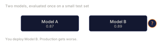
You trained two models. Model A scores 0.87 on your test set. Model B scores 0.89. You deploy Model B. Three weeks later, production metrics are worse than before. What happened?
Model B never actually beat Model A. The 0.02 gap was noise: your test set was too small, the variance too high, or both. You shipped randomness dressed up as improvement.
I've watched this happen constantly. Kaggle leaderboard shakeups. Papers that fail to reproduce. A/B tests that crown a winner off a few hundred samples. The root cause is always the same: someone skipped the statistics.
Statistics is how you tell signal from noise: when a difference is real, how confident to be in it, how much data you need before you trust a result at all. Skip it, and every model comparison you run is a coin flip with extra decimal places.

The Concept
Descriptive Statistics: Summarizing Your Data
Descriptive statistics compress a dataset into a few numbers that capture its shape. Before you model anything, you need to know what your data actually looks like.
Measures of central tendency answer "where is the middle?"
Mean:   sum of all values / count
        mu = (1/n) * sum(x_i)

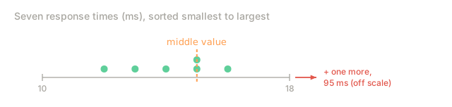
Median: middle value when sorted
        Robust to outliers. If you have [1, 2, 3, 4, 1000], the mean is 202
        but the median is 3.

Mode:   most frequent value
        Useful for categorical data. For continuous data, rarely informative.
The mean is the balance point. The median is the halfway mark. When they diverge, your distribution is skewed. Income distributions have mean >> median (right skew from billionaires). Loss distributions during training often have mean << median (left skew from easy samples).
Measures of spread answer "how dispersed is the data?"
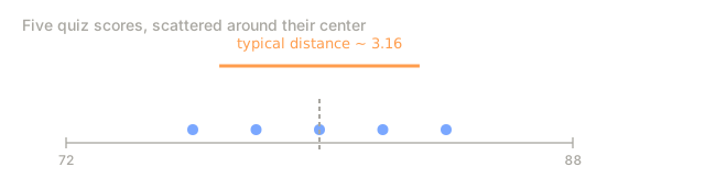
Variance:   average squared deviation from the mean
            sigma^2 = (1/n) * sum((x_i - mu)^2)

Standard deviation:  square root of variance
                     sigma = sqrt(sigma^2)
                     Same units as the data, so more interpretable.

Range:      max - min
            Sensitive to outliers. Almost never useful alone.

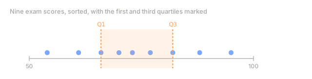
IQR:        Q3 - Q1 (interquartile range)
            The range of the middle 50% of the data.
            Robust to outliers. Used for box plots and outlier detection.
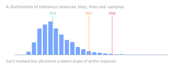
Percentiles divide sorted data into 100 equal parts. The 25th percentile (Q1) means 25% of values fall below this point. The 50th percentile is the median. The 75th percentile is Q3.
For latency monitoring:
  P50 = median latency        (typical user experience)
  P95 = 95th percentile       (bad but not worst case)
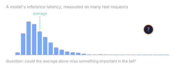
  P99 = 99th percentile       (tail latency, often 10x the median)
In ML, you care about percentiles for inference latency, prediction confidence distributions, and understanding error distributions. A model with low average error but terrible P99 error might be useless for safety-critical applications.
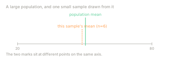
Sample vs population statistics. When computing variance from a sample, divide by (n-1) instead of n. This is Bessel's correction. It compensates for the fact that your sample mean is not the true population mean. With n in the denominator, you systematically underestimate the true variance. With (n-1), the estimate is unbiased.
Population variance: sigma^2 = (1/N) * sum((x_i - mu)^2)
Sample variance:     s^2     = (1/(n-1)) * sum((x_i - x_bar)^2)
In practice: if n is large (thousands of samples), the difference is negligible. If n is small (dozens of samples), it matters.
Correlation: How Variables Move Together
Correlation measures the strength and direction of a linear relationship between two variables.
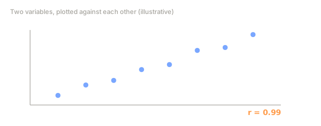
Pearson correlation coefficient measures linear association:
r = sum((x_i - x_bar)(y_i - y_bar)) / (n * s_x * s_y)

r = +1:  perfect positive linear relationship
r = -1:  perfect negative linear relationship
r =  0:  no linear relationship (but there might be a nonlinear one!)

Range: [-1, 1]
Pearson assumes the relationship is linear and both variables are roughly normally distributed. It is sensitive to outliers. A single extreme point can drag r from 0.1 to 0.9.
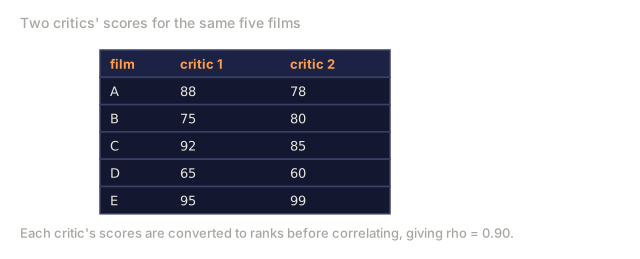
Spearman rank correlation measures monotonic association:
1. Replace each value with its rank (1, 2, 3, ...)
2. Compute Pearson correlation on the ranks

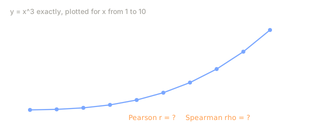
Spearman catches any monotonic relationship, not just linear.
If y = x^3, Pearson gives r < 1 but Spearman gives rho = 1.
When to use each:
Pearson:    Both variables are continuous and roughly normal.
            You care about the linear relationship specifically.
            No extreme outliers.

Spearman:   Ordinal data (rankings, ratings).
            Data is not normally distributed.
            You suspect a monotonic but not linear relationship.
            Outliers are present.
No exceptions: correlation does not imply causation. Ice cream sales and drowning deaths rise together because both track summer. Your model's accuracy and its parameter count move together too, but stacking on more parameters does not automatically buy you accuracy (see: overfitting).
Covariance Matrix
The covariance between two variables measures how they vary together:
Cov(X, Y) = (1/n) * sum((x_i - x_bar)(y_i - y_bar))

Cov(X, Y) > 0:  X and Y tend to increase together
Cov(X, Y) < 0:  when X increases, Y tends to decrease
Cov(X, Y) = 0:  no linear co-movement
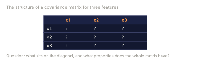
For d features, the covariance matrix C is a d x d matrix where C[i][j] = Cov(feature_i, feature_j). The diagonal entries C[i][i] are the variances of each feature.
C = | Var(x1)      Cov(x1,x2)  Cov(x1,x3) |
    | Cov(x2,x1)  Var(x2)      Cov(x2,x3) |
    | Cov(x3,x1)  Cov(x3,x2)  Var(x3)     |

Properties:
  - Symmetric: C[i][j] = C[j][i]
  - Positive semi-definite: all eigenvalues >= 0
  - Diagonal = variances
  - Off-diagonal = covariances
Connection to PCA. PCA eigendecomposes the covariance matrix. The eigenvectors are the principal components (directions of maximum variance). The eigenvalues tell you how much variance each component captures. This is exactly what Lesson 10 covered, but now you see why the covariance matrix is the right thing to decompose: it encodes all pairwise linear relationships in your data.
Connection to correlation. The correlation matrix is the covariance matrix of standardized variables (each divided by its standard deviation). Correlation normalizes covariance so all values fall in [-1, 1].
Hypothesis Testing
Hypothesis testing is a framework for making decisions under uncertainty. You start with a claim, collect data, and determine if the data is consistent with the claim.
The setup:
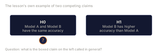
Null hypothesis (H0):        the default assumption, usually "no effect"
Alternative hypothesis (H1): what you are trying to show

Example:
  H0: Model A and Model B have the same accuracy
  H1: Model B has higher accuracy than Model A
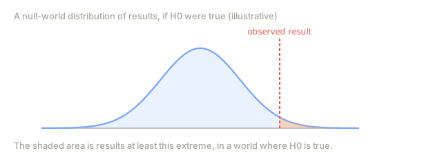
The p-value is the probability of seeing data as extreme as what you observed, assuming H0 is true. It is NOT the probability that H0 is true. This is the single most common misunderstanding in statistics.
p-value = P(data this extreme | H0 is true)

If p-value < alpha (typically 0.05):
    Reject H0. The result is "statistically significant."
If p-value >= alpha:
    Fail to reject H0. You do not have enough evidence.
    This does NOT mean H0 is true.
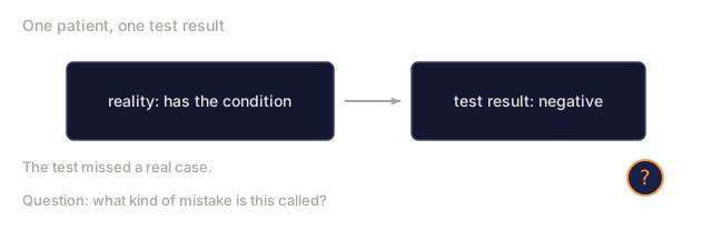
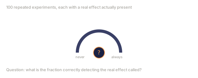
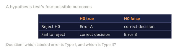
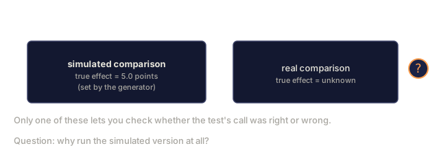
Two ways this decision goes wrong: rejecting H0 when it is actually true (a Type I error, a false positive, at exactly the alpha rate you chose) or failing to reject H0 when it is actually false (a Type II error, a false negative). Statistical power is 1 minus the Type II error rate: the probability you correctly catch a real effect when one exists. Build It's A/B test simulator measures both error rates directly, by running the test against data where you already know the ground truth.
Confidence intervals give a range of plausible values for a parameter:
95% confidence interval for the mean:
    x_bar +/- z * (s / sqrt(n))

where z = 1.96 for 95% confidence

Interpretation: if you repeated this experiment many times, 95% of the
computed intervals would contain the true mean. It does NOT mean there
is a 95% probability the true mean is in this specific interval.
The width of the confidence interval tells you about precision. Wide intervals mean high uncertainty. Narrow intervals mean your estimate is precise (but not necessarily accurate, if your data is biased).
The t-test
The t-test compares means. There are several flavors.
One-sample t-test: is the population mean different from a hypothesized value?
t = (x_bar - mu_0) / (s / sqrt(n))

degrees of freedom = n - 1
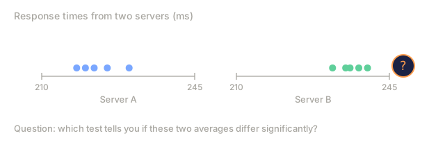
Two-sample t-test (independent): are two group means different?
t = (x_bar_1 - x_bar_2) / sqrt(s1^2/n1 + s2^2/n2)

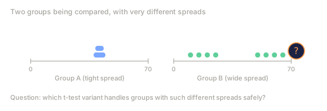
This is Welch's t-test, which does not assume equal variances.
Always use Welch's unless you have a specific reason for equal variances.
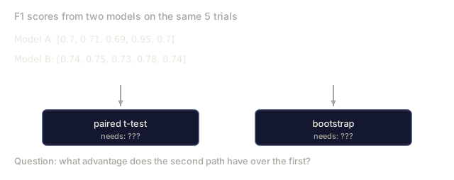
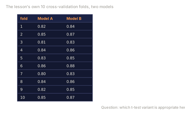
Paired t-test: when measurements come in pairs (same model evaluated on same data splits):
Compute d_i = x_i - y_i for each pair
Then run a one-sample t-test on the d_i values against mu_0 = 0
In ML, the paired t-test is common: you run both models on the same 10 cross-validation folds and compare their scores pairwise.
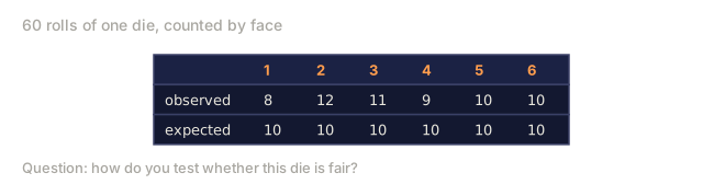
Chi-squared Test
The chi-squared test checks if observed frequencies match expected frequencies. Useful for categorical data.
chi^2 = sum((observed - expected)^2 / expected)

Example: does a language model's output distribution match the
training distribution across categories?

Category    Observed   Expected
Positive       120        100
Negative        80        100
chi^2 = (120-100)^2/100 + (80-100)^2/100 = 4 + 4 = 8

With 1 degree of freedom, chi^2 = 8 gives p < 0.005.
The difference is significant.
A/B Testing for ML Models
A/B testing means comparing two variants against each other under identical conditions to see which one performs better. In ML, that comparison is not the same as a web A/B test: model comparison has specific challenges:
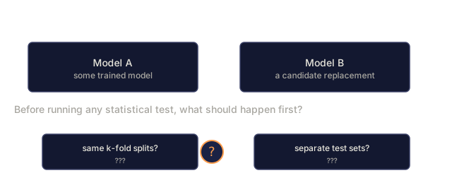
1. Same test set:    Both models must be evaluated on identical data.
                     Different test sets make comparison meaningless.

2. Multiple metrics: Accuracy alone is not enough. You need precision,
                     recall, F1, latency, and fairness metrics.

3. Variance:         Use cross-validation or bootstrap to estimate
                     the variance of each metric, not just point estimates.

4. Data leakage:     If the test set was used during model selection,
                     your comparison is biased. Hold out a final test set.
The procedure:
1. Define your metric and significance level (alpha = 0.05)
2. Run both models on the same k-fold cross-validation splits
3. Collect paired scores: [(a1, b1), (a2, b2), ..., (ak, bk)]
4. Compute differences: d_i = b_i - a_i
5. Run a paired t-test on the differences
6. Check: is the mean difference significantly different from 0?
7. Compute a confidence interval for the mean difference
8. Compute effect size (Cohen's d) to judge practical significance
Statistical Significance vs Practical Significance
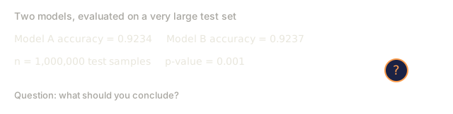
A result can be statistically significant but practically meaningless. With enough data, even a trivial difference becomes statistically significant.
Example:
  Model A accuracy: 0.9234
  Model B accuracy: 0.9237
  n = 1,000,000 test samples
  p-value = 0.001

Statistically significant? Yes.
Practically significant? A 0.03% improvement is not worth the
engineering cost of deploying a new model.
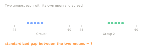
Effect size quantifies how big the difference is, independent of sample size:
Cohen's d = (mean_1 - mean_2) / pooled_std

d = 0.2:  small effect
d = 0.5:  medium effect
d = 0.8:  large effect
Always report both the p-value and the effect size. The p-value tells you if the difference is real. The effect size tells you if it matters.
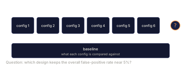
Multiple Comparison Problem
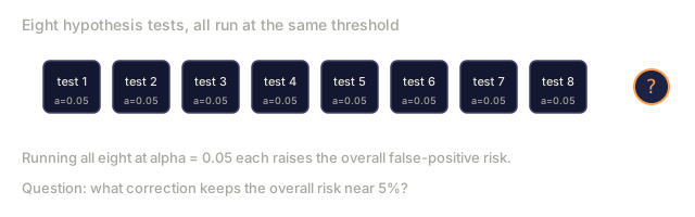
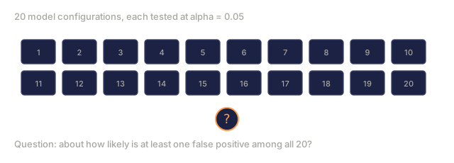
When you test many hypotheses, some will be "significant" by chance. If you test 20 things at alpha = 0.05, you expect 1 false positive even when nothing is real.
P(at least one false positive) = 1 - (1 - alpha)^m

m = 20 tests, alpha = 0.05:
P(false positive) = 1 - 0.95^20 = 0.64

You have a 64% chance of at least one false positive.
Bonferroni correction: divide alpha by the number of tests.
Adjusted alpha = alpha / m = 0.05 / 20 = 0.0025

Only reject H0 if p-value < 0.0025.
Conservative but simple. Works when tests are independent.
In ML, this matters when you compare a model across multiple metrics, test many hyperparameter configurations, or evaluate on multiple datasets.
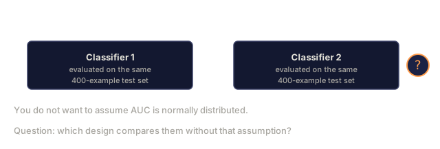
Bootstrap Methods
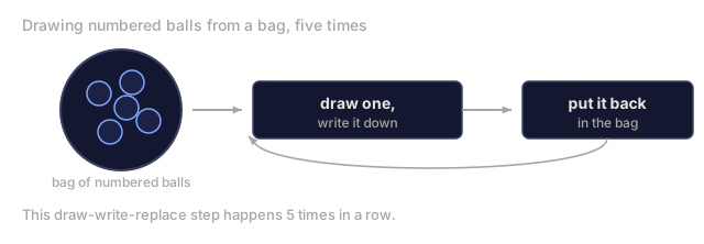
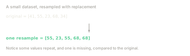
Bootstrapping estimates the sampling distribution of a statistic by resampling your data with replacement. No assumptions about the underlying distribution required.
The algorithm:
1. You have n data points
2. Draw n samples WITH replacement (some points appear multiple times,
   some not at all)
3. Compute your statistic on this bootstrap sample
4. Repeat B times (typically B = 1000 to 10000)
5. The distribution of bootstrap statistics approximates the
   sampling distribution
Bootstrap confidence interval (percentile method):
Sort the B bootstrap statistics
95% CI = [2.5th percentile, 97.5th percentile]
Why bootstrap matters for ML:
- Test set accuracy is a point estimate. Bootstrap gives you
  confidence intervals.
- You cannot assume metric distributions are normal (especially
  for AUC, F1, precision at k).
- Bootstrap works for ANY statistic: median, ratio of two means,
  difference in AUC between two models.
- No closed-form formula needed.
Bootstrap for model comparison:
1. You have predictions from Model A and Model B on the same test set
2. For each bootstrap iteration:
   a. Resample test indices with replacement
   b. Compute metric_A and metric_B on the resampled set
   c. Store diff = metric_B - metric_A
3. 95% CI for the difference:
   [2.5th percentile of diffs, 97.5th percentile of diffs]
4. If the CI does not contain 0, the difference is significant
This is more robust than the paired t-test because it makes no distributional assumptions.
Parametric vs Non-parametric Tests
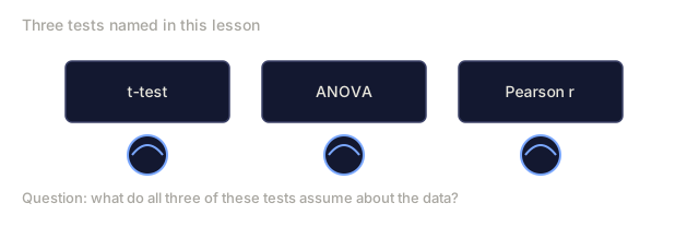
Parametric tests assume a specific distribution (usually normal):
t-test:         assumes normally distributed data (or large n by CLT)
ANOVA:          assumes normality and equal variances
Pearson r:      assumes bivariate normality
Non-parametric tests make no distributional assumptions:
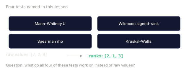
Mann-Whitney U:     compares two groups (replaces independent t-test)
Wilcoxon signed-rank: compares paired data (replaces paired t-test)
Spearman rho:       correlation on ranks (replaces Pearson)
Kruskal-Wallis:     compares multiple groups (replaces ANOVA)
When to use non-parametric:
- Small sample size (n < 30) and data is clearly non-normal
- Ordinal data (ratings, rankings)
- Heavy outliers you cannot remove
- Skewed distributions
When to use parametric:
- Large sample size (CLT makes the test statistic approximately normal)
- Data is roughly symmetric without extreme outliers
- More statistical power (better at detecting real differences)
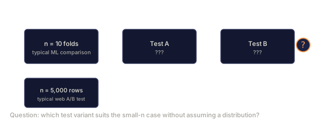
In ML experiments, you typically have small n (5 or 10 cross-validation folds), so non-parametric tests like Wilcoxon signed-rank are often more appropriate than t-tests.
Central Limit Theorem: Practical Implications
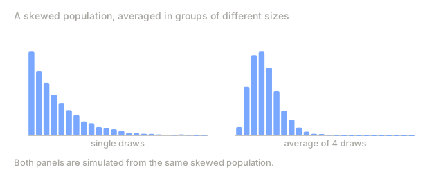
The CLT says the distribution of sample means approaches a normal distribution as n grows, regardless of the underlying population distribution.
If X_1, X_2, ..., X_n are iid with mean mu and variance sigma^2:

    X_bar ~ Normal(mu, sigma^2 / n)    as n -> infinity

Works for n >= 30 in most cases.
For highly skewed distributions, you might need n >= 100.
Why this matters for ML:
1. Justifies confidence intervals and t-tests on aggregated metrics
2. Explains why averaging over cross-validation folds gives stable
   estimates even when individual folds vary wildly
3. Mini-batch gradient descent works because the average gradient
   over a batch approximates the true gradient (CLT in action)
4. Ensemble methods: averaging predictions from many models gives
   more stable output than any single model
What CLT does NOT do:
- Does NOT make your data normal. It makes the MEAN of samples normal.
- Does NOT work for heavy-tailed distributions with infinite variance
  (Cauchy distribution).
- Does NOT apply to dependent data (time series without correction).
Common Statistical Mistakes in ML Papers
-
Testing on the training set. Guarantees overfitting. Always hold out data the model never sees during training.
-
No confidence intervals. Reporting a single accuracy number without uncertainty makes results unreproducible and unverifiable.
-
Ignoring multiple comparisons. Testing 50 configurations and reporting the best one without correction inflates false positive rates.
-
Confusing statistical and practical significance. A p-value of 0.001 on a 0.01% accuracy improvement is not meaningful.
-
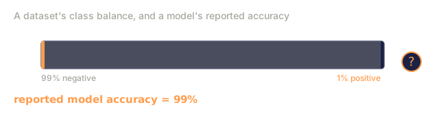
Using accuracy on imbalanced data. 99% accuracy on a dataset with 99% negative class means the model learned nothing. Use precision, recall, F1, or AUC.
-
Cherry-picking metrics. Reporting only the metric where your model wins. Honest evaluation reports all relevant metrics.
-
Leaking information across train/test splits. Normalizing before splitting, or using future data to predict the past.
-
Small test sets with no variance estimates. Evaluating on 100 samples and claiming 2% improvement is noise, not signal.
-
Assuming independence when data is not independent. Medical images from the same patient, multiple sentences from the same document. Observations within a group are correlated.
-
P-hacking. Trying different tests, subsets, or exclusion criteria until you get p < 0.05. The result is an artifact of the search.





Build It
You will implement:
- Descriptive statistics from scratch (mean, median, mode, standard deviation, percentiles, IQR)
- Correlation functions (Pearson and Spearman, with the covariance matrix)
- Hypothesis tests (one-sample t-test, two-sample t-test, chi-squared test)
- Bootstrap confidence intervals (for any statistic, no assumptions needed)
- A/B test simulator (generate data, test, check for Type I and Type II errors)
- Statistical vs practical significance demo (showing that large n makes everything "significant")
All from scratch, using only math and random. No numpy, no scipy. Skipping the libraries here is not busywork: it's the only way to actually know what scipy.stats.ttest_ind is doing before you trust its output on a comparison that decides what ships.
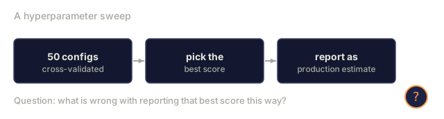
The mistake I see more than any other here isn't a wrong formula. It's losing track of where the test set boundary actually is. Someone runs a hyperparameter sweep, fifty configs, all cross-validated, and reports the best one's score as if that number were an unbiased estimate of production performance. It isn't. Fifty implicit hypothesis tests just ran to find that "best" config, and the multiple comparison problem does not care that you called it a sweep instead of a science experiment.
The fix is boring: hold out a true final test set that no hyperparameter search ever touches, and report your sweep's best result with a bootstrap confidence interval, not a bare number. If that interval is wide, you did not find a better model. You found a lucky seed.
Exercises
- Extend
bootstrap_statisticto also report the bootstrap standard error (the standard deviation of the resampled statistics), not just the percentile CI. Run it on a normal sample and compare that standard error against the closed-forms / sqrt(n). How close are they, and does the gap shrink asn_bootstrapgrows? run_multiple_ab_testsruns m independent comparisons. Measure its observed false-positive rate at m = 20, with and without applyingbonferroni_correctionto the p-values. Does the uncorrected rate land near the 64% this lesson derives analytically?- Pick a small, visibly skewed dataset (5-10 points, one clear outlier). Run
two_sample_tteston it, then implement a bare-bones Wilcoxon signed-rank test and run that too. Do the two tests agree on significance? Which result would you trust more, and why? - Use
ab_test_simulatorto generate two models that differ by a fixed, tiny true effect, once with n = 100 and once with n = 100000. At which sample size doespaired_ttestcall the difference significant? Runcohens_dat both sample sizes and show that the effect size barely moves while the p-value swings from "not significant" to "significant." covariance_matrixreturns covariances. Add acorrelation_matrixfunction that standardizes it (divide each entry by the product of the corresponding standard deviations) and verify the diagonal comes out as all 1s on any dataset you feed it.
Key Terms
| Term | Definition |
|---|---|
| Mean | Sum of values divided by count. Sensitive to outliers. |
| Median | Middle value of sorted data. Robust to outliers. |
| Standard deviation | Square root of variance. Measures spread in original units. |
| Percentile | Value below which a given percentage of data falls. |
| IQR | Interquartile range. Q3 minus Q1. The spread of the middle 50%. |
| Pearson correlation | Measures linear association between two variables. Range [-1, 1]. |
| Spearman correlation | Measures monotonic association using ranks. |
| Covariance matrix | Matrix of pairwise covariances between all features. |
| Null hypothesis | Default assumption of no effect or no difference. |
| p-value | Probability of data this extreme given the null hypothesis is true. |
| Confidence interval | Range of plausible values for a parameter at a given confidence level. |
| t-test | Tests whether means differ significantly. Uses the t-distribution. |
| Chi-squared test | Tests whether observed frequencies differ from expected frequencies. |
| Effect size | Magnitude of a difference, independent of sample size. Cohen's d is common. |
| Bonferroni correction | Divides significance threshold by number of tests to control false positives. |
| Bootstrap | Resampling with replacement to estimate sampling distributions. |
| Type I error | False positive. Rejecting H0 when it is true. |
| Type II error | False negative. Failing to reject H0 when it is false. |
| Statistical power | Probability of correctly rejecting a false H0. Power = 1 minus Type II error rate. |
| Central limit theorem | Sample means converge to a normal distribution as sample size grows. |
| Parametric test | Assumes a specific distribution for the data (usually normal). |
| Non-parametric test | Makes no distributional assumptions. Works on ranks or signs. |
Code
- statistics.py (python, 619 lines)