Bayes' Theorem
Probability is about what you expect. Bayes' theorem is about what you learn.
Learning Objectives
- Apply Bayes' theorem to compute posterior probabilities from priors, likelihoods, and evidence
- Build a Naive Bayes text classifier from scratch with Laplace smoothing and log-space computation
- Compare MLE and MAP estimation and explain how MAP corresponds to L2 regularization
- Implement sequential Bayesian updating using Beta-Binomial conjugate priors for A/B testing
The Problem
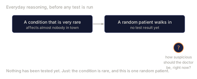
A medical test is 99% accurate. You test positive. What are the chances you actually have the disease?
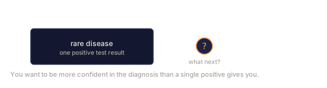
Most people say 99%. The real answer depends on how rare the disease is: if 1 in 10,000 people have it, a positive result only gives you about a 1% chance of being sick. The other 99% of positive results are false alarms from healthy people.
That reasoning is Bayes' theorem, not a trick question. Every spam filter, every medical diagnostic, and every ML model that quantifies uncertainty runs on it: start with a belief, see evidence, update.
Skip this and you'll misread model outputs, set bad thresholds, and ship predictions that are far more confident than the evidence supports.
The Concept
From joint probability to Bayes
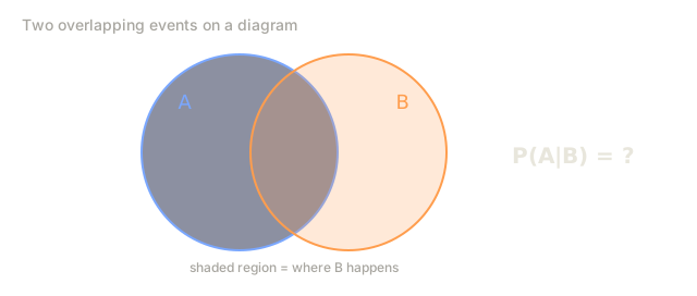
You already know from Lesson 06 that conditional probability is:
P(A|B) = P(A and B) / P(B)
And symmetrically:
P(B|A) = P(A and B) / P(A)
Both expressions share the same numerator: P(A and B). Set them equal and rearrange:
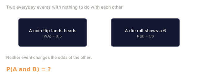
P(A and B) = P(A|B) * P(B) = P(B|A) * P(A)

Therefore:

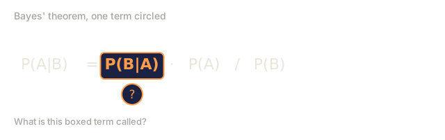
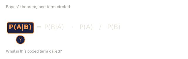
P(A|B) = P(B|A) * P(A) / P(B)
That's Bayes' theorem: four quantities, one equation.
The four parts
| Part | Name | What it means |
|---|---|---|
| P(A|B) | Posterior | Your updated belief about A after seeing evidence B |
| P(B|A) | Likelihood | How probable the evidence B is if A is true |
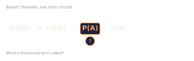
| P(A) | Prior | Your belief about A before seeing any evidence |
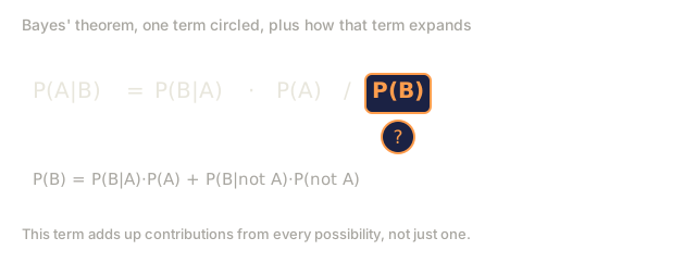
| P(B) | Evidence | Total probability of seeing B under all possibilities |
The evidence term P(B) acts as a normalizer. You can expand it using the law of total probability:
P(B) = P(B|A) * P(A) + P(B|not A) * P(not A)
Medical test example
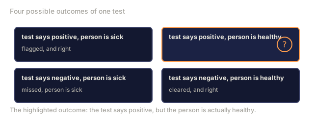
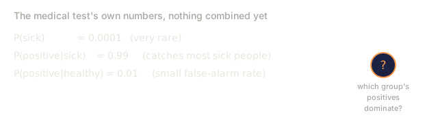
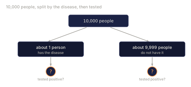
A disease affects 1 in 10,000 people. The test is 99% accurate (catches 99% of sick people, gives false positives 1% of the time).
P(sick)          = 0.0001     (prior: disease is rare)
P(positive|sick) = 0.99       (likelihood: test catches it)
P(positive|healthy) = 0.01    (false positive rate)

P(positive) = P(positive|sick) * P(sick) + P(positive|healthy) * P(healthy)
            = 0.99 * 0.0001 + 0.01 * 0.9999
            = 0.000099 + 0.009999
            = 0.010098

P(sick|positive) = P(positive|sick) * P(sick) / P(positive)
                 = 0.99 * 0.0001 / 0.010098
                 = 0.0098
                 = 0.98%
Less than 1%. The prior dominates. When a condition is rare, even accurate tests produce mostly false positives. This is why doctors order confirmation tests.
Spam filter example
You receive an email containing the word "lottery". Is it spam?
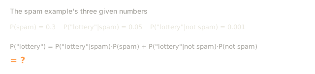
P(spam)                = 0.3      (30% of email is spam)
P("lottery"|spam)      = 0.05     (5% of spam emails contain "lottery")
P("lottery"|not spam)  = 0.001    (0.1% of legitimate emails contain "lottery")

P("lottery") = 0.05 * 0.3 + 0.001 * 0.7
             = 0.015 + 0.0007
             = 0.0157

P(spam|"lottery") = 0.05 * 0.3 / 0.0157
                  = 0.955
                  = 95.5%
One word shifts the probability from 30% to 95.5%. A real spam filter applies Bayes across hundreds of words simultaneously.
Naive Bayes: independence assumption
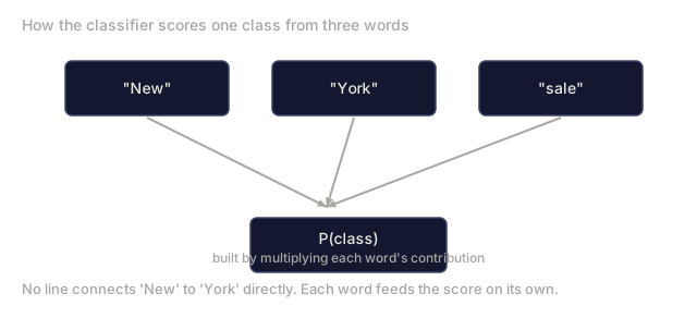
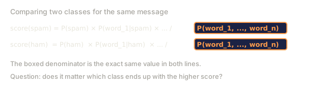
Naive Bayes extends this to multiple features by assuming all features are conditionally independent given the class:
P(class | feature_1, feature_2, ..., feature_n)
  = P(class) * P(feature_1|class) * P(feature_2|class) * ... * P(feature_n|class)
    / P(feature_1, feature_2, ..., feature_n)
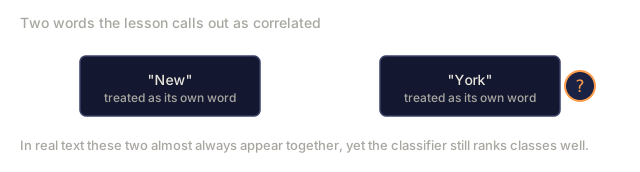
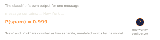
The "naive" part is the independence assumption. In text, word occurrences are not independent ("New" and "York" are correlated). But the assumption works surprisingly well in practice because the classifier only needs to rank classes, not produce calibrated probabilities.
Since the denominator is the same for all classes, you can skip it and just compare numerators:
score(class) = P(class) * product of P(feature_i | class)
Pick the class with the highest score.
Maximum likelihood estimation (MLE)
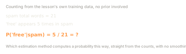
Maximum likelihood estimation picks the parameter values that make the observed data most likely: you're maximizing the likelihood function, and for discrete counts that maximization reduces to plain relative frequency. So how do you get P(feature|class) from training data? Count.
P("free"|spam) = (number of spam emails containing "free") / (total spam emails)
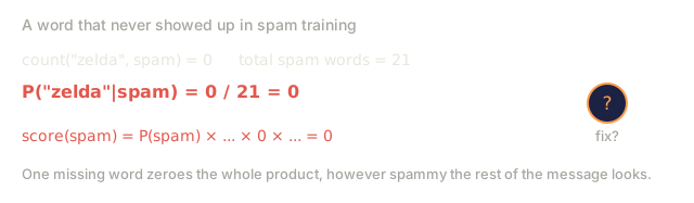
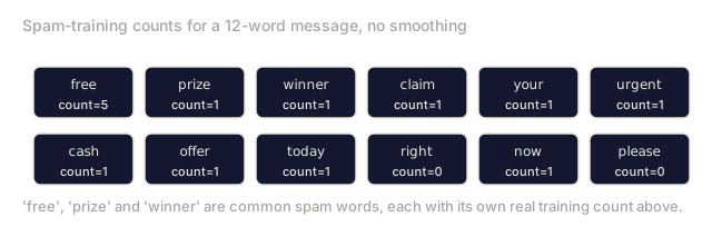
One problem: if a word never appears in spam during training, MLE assigns it probability zero, and one unseen word kills the entire product. Laplace smoothing fixes that:
P(word|class) = (count(word, class) + 1) / (total_words_in_class + vocabulary_size)
Adding 1 to every count guarantees no probability ever hits zero.
Maximum a posteriori (MAP)
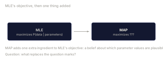
MLE asks: what parameters maximize P(data|parameters)?
MAP asks: what parameters maximize P(parameters|data)?
By Bayes' theorem:
P(parameters|data) proportional to P(data|parameters) * P(parameters)
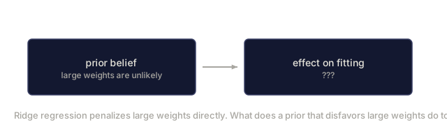
MAP adds a prior over the parameters themselves: if you believe parameters should be small, you encode that as a prior that penalizes large values. That's identical to L2 regularization in ML. The "ridge" penalty in ridge regression is literally a Gaussian prior on the weights.
| Estimation | Optimizes | ML equivalent |
|---|---|---|
| MLE | P(data|params) | Unregularized training |
| MAP | P(data|params) * P(params) | L2 / L1 regularization |
Bayesian vs frequentist: the practical difference
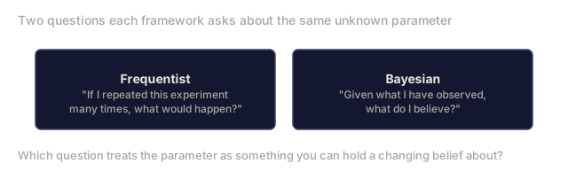
Frequentists treat parameters as fixed unknowns. They ask: "If I repeated this experiment many times, what would happen?"
Bayesians treat parameters as distributions. They ask: "Given what I have observed, what do I believe about the parameters?"
For building ML systems, the practical difference:
| Aspect | Frequentist | Bayesian |
|---|---|---|
| Output | Point estimate | Distribution over values |
| Uncertainty | Confidence intervals (about procedure) | Credible intervals (about parameter) |
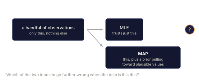
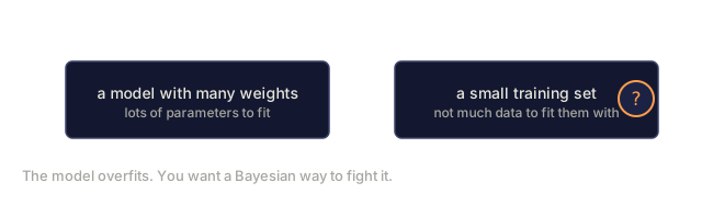
| Small data | Can overfit | Prior acts as regularization |
| Computation | Usually faster | Often requires sampling (MCMC) |
Most production ML is frequentist (SGD, point estimates). Bayesian methods shine when you need calibrated uncertainty (medical decisions, safety-critical systems) or when data is scarce (few-shot learning, cold start).
Why Bayesian thinking matters for ML
The connection is deeper than analogy:
Priors are regularization. A Gaussian prior on weights is L2 regularization. A Laplace prior is L1. Every time you add a regularization term, you are making a Bayesian statement about what parameter values you expect.
Posteriors are uncertainty. A single predicted probability tells you nothing about how confident the model is in that estimate. Bayesian methods give you a distribution: "I think P(spam) is between 0.8 and 0.95."
Bayes updates are online learning. Today's posterior becomes tomorrow's prior. When your model sees new data, it updates its beliefs incrementally instead of retraining from scratch.
Model comparison is Bayesian. Bayesian information criterion (BIC), marginal likelihood, and Bayes factors all use Bayesian reasoning to choose between models without overfitting.
Conjugate priors
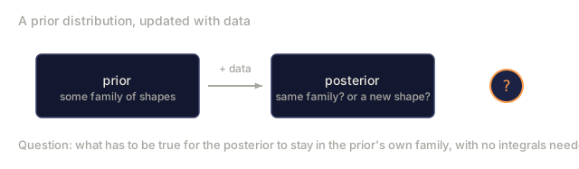
When the prior and posterior belong to the same family of distributions, the prior is called "conjugate." That makes Bayesian updating algebraically clean: you get a closed-form posterior without numerical integration.
| Likelihood | Conjugate Prior | Posterior | Example |
|---|---|---|---|
| Bernoulli | Beta(a, b) | Beta(a + successes, b + failures) | Coin flip bias estimation |
| Normal (known variance) | Normal(mu_0, sigma_0) | Normal(weighted mean, smaller variance) | Sensor calibration |
| Poisson | Gamma(a, b) | Gamma(a + sum of counts, b + n) | Modeling arrival rates |
| Multinomial | Dirichlet(alpha) | Dirichlet(alpha + counts) | Topic modeling, language models |
The Beta row is the one this lesson uses below. The others are worth recognizing by name when you meet them later: Gamma models rates and waiting times, Dirichlet is just Beta generalized past two outcomes.
Without a conjugate prior, you need Monte Carlo sampling or variational inference to approximate the posterior. With one, you just update two numbers.
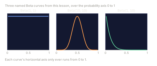
Beta(a, b) represents your belief about a probability parameter. Its mean is a/(a+b), and the larger a+b gets, the more concentrated (confident) the distribution is:
- Beta(1, 1) = uniform. You have no opinion about the parameter.
- Beta(10, 10) = peaked at 0.5. You strongly believe the parameter is near 0.5.
- Beta(1, 10) = skewed toward 0. You believe the parameter is small.
The update rule is dead simple:
Prior:     Beta(a, b)
Data:      s successes, f failures
Posterior: Beta(a + s, b + f)
No integrals. No sampling. Just addition.
Sequential Bayesian updating
Bayesian inference is naturally sequential. Today's posterior becomes tomorrow's prior. This is how real systems learn incrementally without reprocessing all historical data.
Concrete example: estimating whether a coin is fair.
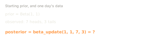
Day 1: No data yet. Start with Beta(1, 1), a uniform prior. You have no opinion.
- Prior mean: 0.5
- Prior is flat across [0, 1]
Day 2: Observe 7 heads, 3 tails. Posterior = Beta(1 + 7, 1 + 3) = Beta(8, 4)
- Posterior mean: 8/12 = 0.667
- Evidence suggests the coin is biased toward heads
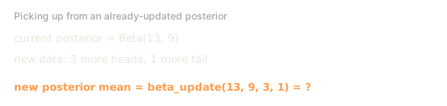
Day 3: Observe 5 more heads, 5 more tails. Use yesterday's posterior as today's prior. Posterior = Beta(8 + 5, 4 + 5) = Beta(13, 9)
- Posterior mean: 13/22 = 0.591
- The balanced new data pulled the estimate back toward 0.5

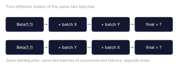
The order of observations doesn't matter: Beta(1,1) updated with all 12 heads and 8 tails at once gives Beta(13, 9), the same result. Sequential updating and batch updating are mathematically equivalent, but sequential updating lets you make decisions at each step without storing raw data.
This is the foundation of online learning in production ML systems. Thompson sampling for bandits, incremental recommendation systems, and streaming anomaly detectors all use this pattern.
Connection to A/B testing
A/B testing is Bayesian inference in disguise: you are estimating two conversion rates and asking which one is actually higher.
Setup: you are testing two button colors. Variant A (blue) and variant B (green). You want to know which one gets more clicks.
The Bayesian A/B test:
- Prior. Start with Beta(1, 1) for both variants. No prior preference.
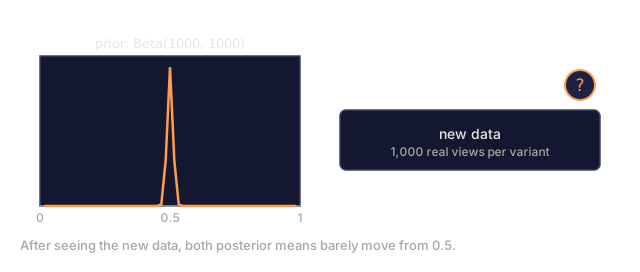
- Data. Variant A: 50 clicks out of 1000 views. Variant B: 65 clicks out of 1000 views.
- Posteriors.
- A: Beta(1 + 50, 1 + 950) = Beta(51, 951). Mean = 0.051
- B: Beta(1 + 65, 1 + 935) = Beta(66, 936). Mean = 0.066
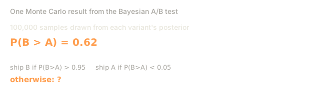
- Decision. Compute P(B > A): the probability that B's true conversion rate is higher than A's.
Computing P(B > A) analytically is hard. But Monte Carlo makes it trivial:
1. Draw 100,000 samples from Beta(51, 951)  -> samples_A
2. Draw 100,000 samples from Beta(66, 936)  -> samples_B
3. P(B > A) = fraction of samples where B > A
If P(B > A) > 0.95, you ship variant B. If it is between 0.05 and 0.95, you keep collecting data. If P(B > A) < 0.05, you ship variant A.
Advantages over frequentist A/B testing:
- You get a direct probability statement: "there is a 97% chance B is better"
- No p-value confusion. No "fail to reject the null hypothesis" hedging.
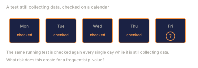
- You can check results at any time without inflating false positive rates (no "peeking problem")
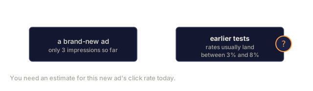
- You can incorporate prior knowledge (e.g., previous tests suggest conversion rates are usually 3-8%)
| Aspect | Frequentist A/B | Bayesian A/B |
|---|---|---|
| Output | p-value | P(B > A) |
| Interpretation | "How surprising is this data if A=B?" | "How likely is B better than A?" |
| Early stopping | Inflates false positives | Safe at any point (given a well-chosen prior and correctly specified model) |
| Prior knowledge | Not used | Encoded as Beta prior |
| Decision rule | p < 0.05 | P(B > A) > threshold |
Build It
Step 1: Bayes theorem function
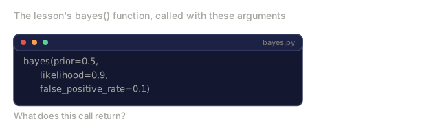
def bayes(prior, likelihood, false_positive_rate):
    evidence = likelihood * prior + false_positive_rate * (1 - prior)
    posterior = likelihood * prior / evidence
    return posterior

result = bayes(prior=0.0001, likelihood=0.99, false_positive_rate=0.01)
print(f"P(sick|positive) = {result:.4f}")
Step 2: Naive Bayes classifier
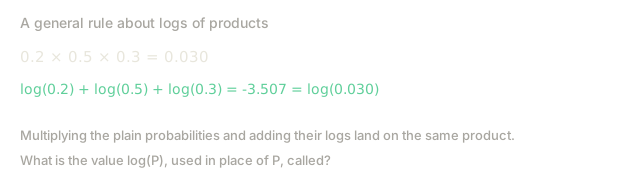
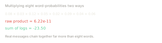
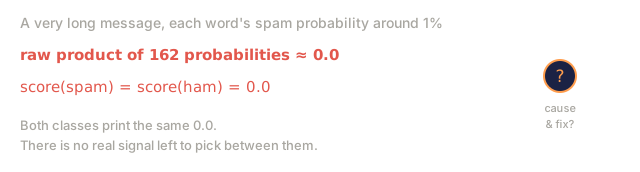
A real message drags dozens of word probabilities into one product, and multiplying that many small numbers together underflows to zero long before you reach the end. So this classifier accumulates scores in log space instead: summing log-probabilities is numerically stable and produces the same ranking multiplying the raw probabilities would.
import math
from collections import defaultdict

class NaiveBayes:
    def __init__(self, smoothing=1.0):
        self.smoothing = smoothing
        self.class_counts = defaultdict(int)
        self.word_counts = defaultdict(lambda: defaultdict(int))
        self.class_word_totals = defaultdict(int)
        self.vocab = set()

    def train(self, documents, labels):
        for doc, label in zip(documents, labels):
            self.class_counts[label] += 1
            words = doc.lower().split()
            for word in words:
                self.word_counts[label][word] += 1
                self.class_word_totals[label] += 1
                self.vocab.add(word)

    def predict(self, document):
        words = document.lower().split()
        total_docs = sum(self.class_counts.values())
        vocab_size = len(self.vocab)
        best_class = None
        best_score = float("-inf")
        for cls in self.class_counts:
            score = math.log(self.class_counts[cls] / total_docs)
            for word in words:
                count = self.word_counts[cls].get(word, 0)
                total = self.class_word_totals[cls]
                score += math.log((count + self.smoothing) / (total + self.smoothing * vocab_size))
            if score > best_score:
                best_score = score
                best_class = cls
        return best_class
Step 3: Train on spam data
train_docs = [
    "win free money now",
    "free lottery ticket winner",
    "claim your prize today free",
    "urgent offer free cash",
    "congratulations you won free",
    "meeting tomorrow at noon",
    "project update attached",
    "can we schedule a call",
    "quarterly report review",
    "lunch on thursday sounds good",
    "team standup notes attached",
    "please review the pull request",
]

train_labels = [
    "spam", "spam", "spam", "spam", "spam",
    "ham", "ham", "ham", "ham", "ham", "ham", "ham",
]

classifier = NaiveBayes()
classifier.train(train_docs, train_labels)

test_messages = [
    "free money waiting for you",
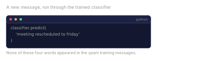
    "meeting rescheduled to friday",
    "you won a free prize",
    "please review the attached report",
]

for msg in test_messages:
    print(f"  '{msg}' -> {classifier.predict(msg)}")
Step 4: Inspect the learned probabilities
def show_top_words(classifier, cls, n=5):
    vocab_size = len(classifier.vocab)
    total = classifier.class_word_totals[cls]
    probs = {}
    for word in classifier.vocab:
        count = classifier.word_counts[cls].get(word, 0)
        probs[word] = (count + classifier.smoothing) / (total + classifier.smoothing * vocab_size)
    sorted_words = sorted(probs.items(), key=lambda x: x[1], reverse=True)
    for word, prob in sorted_words[:n]:
        print(f"    {word}: {prob:.4f}")

print("\nTop spam words:")
show_top_words(classifier, "spam")
print("\nTop ham words:")
show_top_words(classifier, "ham")
Step 5: Beta-Binomial conjugate updates
The conjugate-prior update from the Concept section is two additions. Here it is as code, applied to the same coin-bias walkthrough:
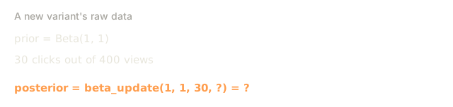
def beta_update(alpha, beta_param, successes, failures):
    return alpha + successes, beta_param + failures

alpha, beta_param = 1, 1  # Beta(1, 1): uniform prior, Day 1 in the walkthrough above
for successes, failures in [(7, 3), (5, 5)]:  # Day 2, then Day 3
    alpha, beta_param = beta_update(alpha, beta_param, successes, failures)
    mean = alpha / (alpha + beta_param)
    print(f"Posterior: Beta({alpha}, {beta_param}), mean = {mean:.4f}")
# -> Beta(8, 4), mean = 0.6667
# -> Beta(13, 9), mean = 0.5909
Each call folds one day's evidence into the running (alpha, beta) pair, reproducing the same two posteriors from the walkthrough above. Feed both batches in at once instead of one at a time and beta_update lands on the same final (alpha, beta): the sequential-equals-batch property from the Concept section.
Step 6: Bayesian A/B test with Monte Carlo
Computing P(B > A) in closed form is hard, but sampling from each variant's Beta posterior and comparing the draws is not:
import random

a_clicks, a_views = 50, 1000
b_clicks, b_views = 65, 1000

a_alpha, a_beta = 1 + a_clicks, 1 + (a_views - a_clicks)
b_alpha, b_beta = 1 + b_clicks, 1 + (b_views - b_clicks)

n_samples = 100_000
b_wins = sum(
    random.betavariate(b_alpha, b_beta) > random.betavariate(a_alpha, a_beta)
    for _ in range(n_samples)
)
print(f"P(B > A) = {b_wins / n_samples:.4f}")
random.betavariate is the stdlib version of the same Beta sampler. The from-scratch implementation in code/bayes.py builds its own (_beta_sample, _gamma_sample) to keep the whole file dependency-free, which is worth reading once to see that a Beta sampler is not magic, but the standard library call above is what you would actually reach for.

Use It
Scikit-learn ships production-ready naive Bayes implementations:
from sklearn.feature_extraction.text import CountVectorizer
from sklearn.naive_bayes import MultinomialNB
from sklearn.metrics import classification_report

vectorizer = CountVectorizer()
X_train = vectorizer.fit_transform(train_docs)
clf = MultinomialNB()
clf.fit(X_train, train_labels)

X_test = vectorizer.transform(test_messages)
predictions = clf.predict(X_test)
for msg, pred in zip(test_messages, predictions):
    print(f"  '{msg}' -> {pred}")
Same algorithm. CountVectorizer handles tokenization and vocabulary building. MultinomialNB handles smoothing and log-probabilities internally. Your from-scratch version does the same thing in 40 lines.
Ship It
The NaiveBayes class built here demonstrates the full pipeline: tokenization, probability estimation with Laplace smoothing, log-space prediction, plus the Beta-Binomial updater and Monte Carlo A/B test from Steps 5 and 6. The code in code/bayes.py runs all of it end-to-end with no dependencies beyond Python's standard library.
The Beta-Binomial update you just built is the same math behind Thompson sampling and online bandit algorithms. You'll meet it again when this curriculum reaches reinforcement learning.
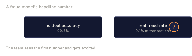
The version of this trap I've actually watched happen isn't a medical test, it's a fraud model. A team ships a classifier that hits 99.5% accuracy on holdout data and gets excited, forgetting to check the base rate: real fraud might be 0.1% of transactions. Flip the confusion matrix and a model can hit that headline number while still missing almost every real fraud case, because predicting "not fraud" for everything already gets you 99.9% accuracy for free. The fix is never a smarter model. It's asking what the prior actually is before you trust the number on the dashboard.
The same trap shows up in A/B tests wearing a different costume. Someone checks the dashboard on day two, sees a 4% lift, and wants to ship. That's peeking, and it's exactly what the Bayesian framing in this lesson is built to survive: with a real posterior instead of a p-value, checking early doesn't lie to you the way frequentist significance testing does.
Exercises
-
Multiple tests. A patient tests positive twice on independent tests (both 99% accurate, disease prevalence 1 in 10,000). What is P(sick) after both tests? Use the posterior from the first test as the prior for the second.
-
Smoothing impact. Run the spam classifier with smoothing values of 0.01, 0.1, 1.0, and 10.0. How do the top word probabilities change? What happens with smoothing=0 and a word that appears only in ham?
-
Add features. Extend the NaiveBayes class to also use message length (short/long) as a feature alongside word counts. Estimate P(short|spam) and P(short|ham) from the training data and fold it into the prediction score.
-
MAP by hand. Given observed data (7 heads in 10 coin flips), compute the MAP estimate of the bias using a Beta(2,2) prior. Compare it to the MLE estimate (7/10).
Key Terms
| Term | What people say | What it actually means |
|---|---|---|
| Prior | "My initial guess" | P(hypothesis) before observing evidence. In ML: the regularization term. |
| Likelihood | "How well the data fits" | P(evidence|hypothesis). How probable the observed data is under a specific hypothesis. |
| Posterior | "My updated belief" | P(hypothesis|evidence). The prior multiplied by the likelihood, then normalized. |
| Evidence | "The normalizing constant" | P(data) across all hypotheses. Ensures the posterior sums to 1. |
| Naive Bayes | "That simple text classifier" | A classifier that assumes features are independent given the class. Works well despite the false assumption. |
| Laplace smoothing | "Add-one smoothing" | Adding a small count to every feature to prevent zero probabilities from unseen data. |
| MLE | "Just use the frequencies" | Choose parameters that maximize P(data|parameters). No prior. Can overfit with small data. |
| MAP | "MLE with a prior" | Choose parameters that maximize P(data|parameters) * P(parameters). Equivalent to regularized MLE. |
| Log-probability | "Work in log space" | Using log(P) instead of P to avoid floating-point underflow when multiplying many small numbers. |
| False positive | "A wrong alarm" | The test says positive, but the true state is negative. Drives the base rate fallacy. |
| Conjugate prior | "The tidy prior" | A prior whose posterior stays in the same distribution family, giving a closed-form update with no sampling. |
| Beta distribution | "The coin-bias curve" | Beta(a, b): a distribution over a probability itself, mean a/(a+b). The conjugate prior for Bernoulli/Binomial data. |
Further Reading
- 3Blue1Brown: Bayes' theorem - visual explanation with the medical test example
- Stanford CS229: Generative Learning Algorithms - naive Bayes and its connection to discriminative models
- Think Bayes - free book, Bayesian statistics with Python code
- scikit-learn Naive Bayes - production implementations and when to use each variant
Code
- bayes.py (python, 346 lines)