Optimization
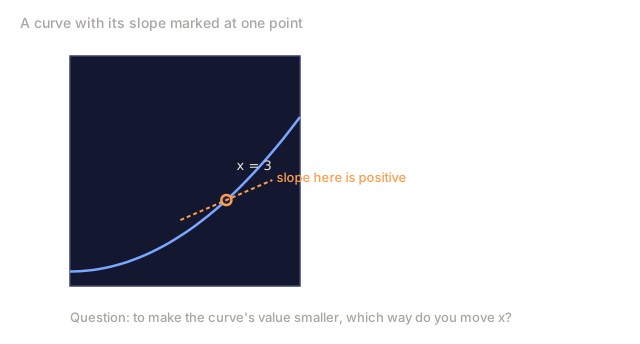
Training a neural network is walking downhill until you hit the bottom of the valley. How you walk is the entire job.
Learning Objectives
- Implement vanilla gradient descent, SGD with momentum, and Adam from scratch
- Compare optimizer convergence on the Rosenbrock function and explain why Adam adapts per-weight learning rates
- Distinguish convex from non-convex loss landscapes and explain the role of saddle points in high dimensions
- Configure learning rate schedules (step decay, cosine annealing, warmup) for training stability
The Problem
You have a loss function that tells you how wrong your model is, and gradients that tell you which direction makes it worse. Now you need a strategy for walking downhill.
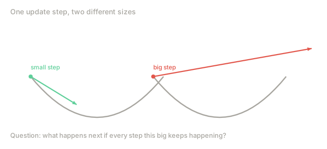
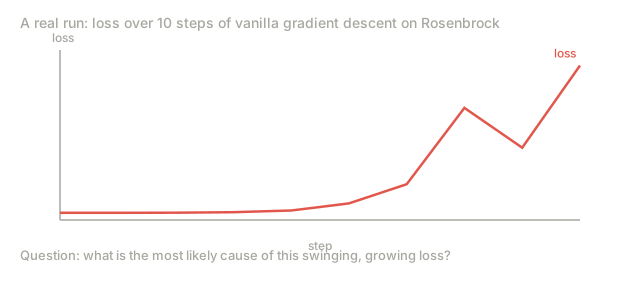
The naive approach is simple: move opposite the gradient, scale the step by some number called the learning rate, and repeat. This is gradient descent, and it works, but "works" has caveats. Too large a learning rate and you overshoot the valley entirely, bouncing between walls. Too small and you crawl toward the answer over thousands of unnecessary steps. Hit a saddle point and you stop moving even though you haven't found a minimum.
Every optimizer in deep learning answers the same question: how do you get to the bottom of the valley faster and more reliably?
The Concept
What optimization means
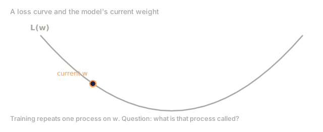
Optimization is finding the input values that minimize (or maximize) a function. In machine learning, the function is the loss. The inputs are the model's weights. Training is optimization.
minimize L(w) where:
  L = loss function
  w = model weights (could be millions of parameters)
Gradient descent (vanilla)
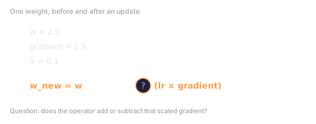
The simplest optimizer. Compute the gradient of the loss with respect to every weight. Move each weight in the opposite direction of its gradient. Scale the step by the learning rate.
w = w - lr * gradient
That is the entire algorithm. One line.

Learning rate: the most important hyperparameter
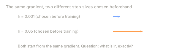
The learning rate is a hyperparameter: a value you choose before training rather than one the model learns. It controls the step size of every update, and it determines nearly everything about whether training converges.

There is no formula for the right learning rate. You find it by experiment. Common starting points: 0.001 for Adam, 0.01 for SGD with momentum.
SGD vs batch vs mini-batch
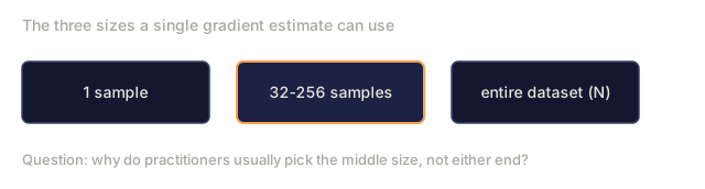
Vanilla gradient descent computes the gradient over the entire dataset before taking a single step. That's called batch gradient descent: stable, but slow.
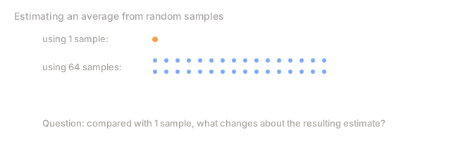
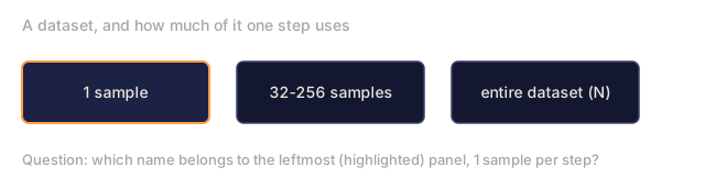
SGD, short for stochastic gradient descent, computes the gradient on one random sample and steps immediately. Noisy, but fast.
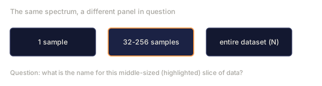
Mini-batch gradient descent splits the difference: compute the gradient over a small batch (32, 64, 128, 256 samples), then step. This is what everyone actually uses in practice.
| Variant | Batch size | Gradient quality | Speed per step | Noise |
|---|---|---|---|---|
| Batch GD | Entire dataset | Exact | Slow | None |
| SGD | 1 sample | Very noisy | Fast | High |
| Mini-batch | 32-256 | Good estimate | Balanced | Moderate |
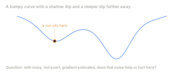
The noise in SGD and mini-batch is not a bug. It helps escape shallow local minima and saddle points.
Momentum: the ball rolling downhill
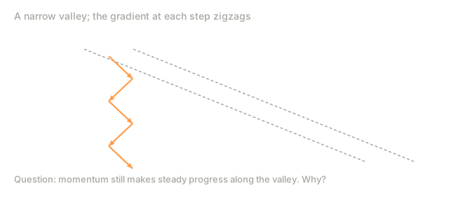
Momentum accumulates past gradients into a velocity term instead of reacting only to the current gradient. That fixes the main weakness of vanilla gradient descent: when the gradient zigzags, which is common in narrow valleys, progress slows to a crawl.
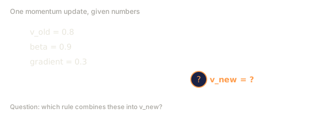
v = beta * v + gradient
w = w - lr * v
The analogy: a ball rolling downhill. It does not stop and restart at every bump. It builds speed in consistent directions and dampens oscillations.

beta (typically 0.9) controls how much history to keep. Higher beta means more momentum, smoother paths, but slower response to direction changes.
Adam: adaptive learning rates
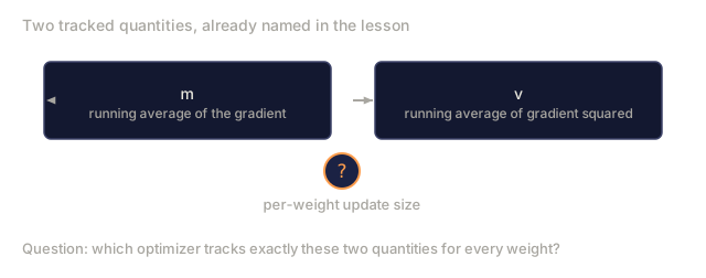
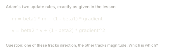
Adam (Adaptive Moment Estimation) tracks two things per weight:
- First moment (m): running average of gradients (like momentum)
- Second moment (v): running average of squared gradients (gradient magnitude)
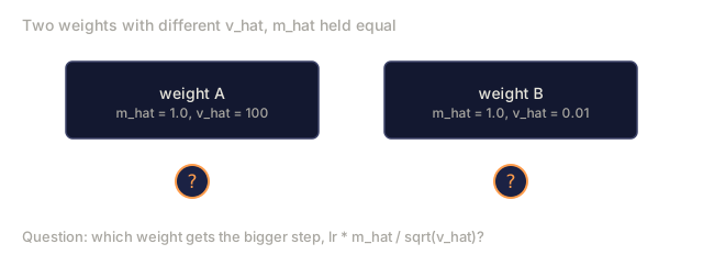
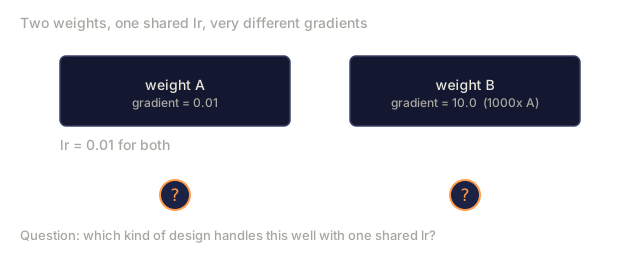
The second moment is what makes the learning rate adaptive per weight: different weights need different step sizes. A weight that rarely gets large gradients should take bigger steps when it finally does. A weight that gets huge gradients constantly should take smaller steps.
m = beta1 * m + (1 - beta1) * gradient
v = beta2 * v + (1 - beta2) * gradient^2

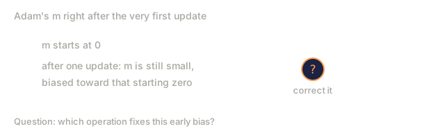
m_hat = m / (1 - beta1^t)    bias correction
v_hat = v / (1 - beta2^t)    bias correction

w = w - lr * m_hat / (sqrt(v_hat) + epsilon)
The division by sqrt(v_hat) is the key insight. Weights with large gradients get divided by a large number (small effective step). Weights with small gradients get divided by a small number (large effective step). Each weight gets its own adaptive learning rate.
Default hyperparameters: lr=0.001, beta1=0.9, beta2=0.999, epsilon=1e-8. These defaults work well for most problems.
Learning rate schedules
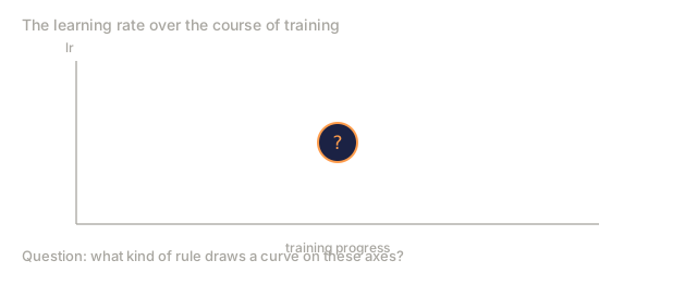
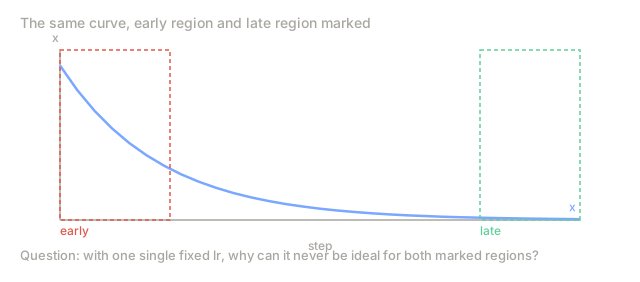
A learning rate schedule changes the learning rate as training progresses instead of holding it fixed. A fixed rate is always a compromise: early in training you want large steps for fast progress, late in training you want small steps to fine-tune near the minimum.
Common schedules:
| Schedule | Formula | Use case |
|---|---|---|
| Step decay | lr = lr * factor every N epochs | Simple, manual control |
| Exponential decay | lr = lr_0 * decay^t | Smooth reduction |
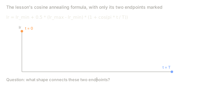
| Cosine annealing | lr = lr_min + 0.5 * (lr_max - lr_min) * (1 + cos(pi * t / T)) | Transformers, modern training |
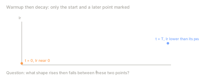
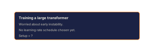
| Warmup + decay | Linear ramp up, then decay | Large models, prevents early instability |
An epoch is one full pass through the training set. Step decay and similar schedules count in epochs; the loop you built in Build It counts in raw optimizer steps instead. Same idea, different unit.
Convex vs non-convex
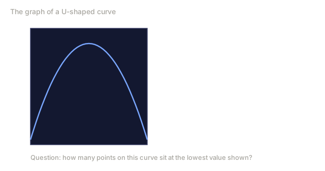
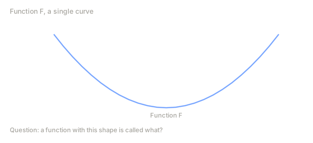
A convex function has one minimum. Gradient descent always finds it. A quadratic like f(x) = x^2 is convex.
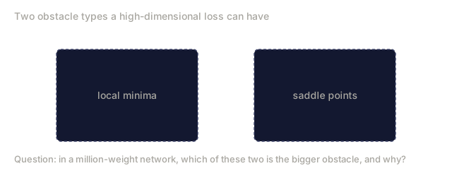
Neural network loss functions are non-convex. They have many local minima, saddle points, and flat regions.

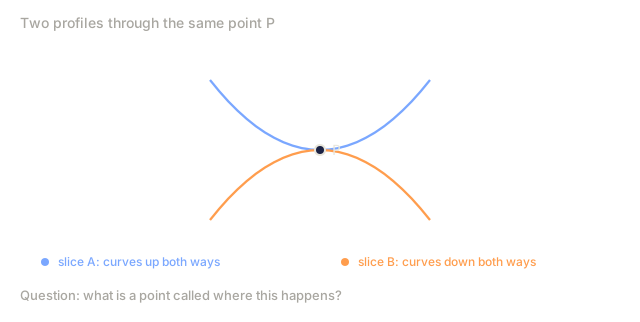
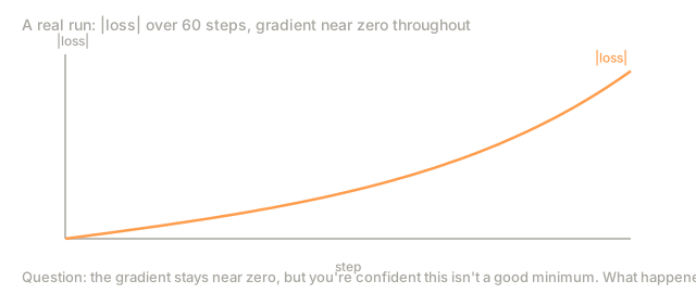
In practice, local minima in high-dimensional neural networks are rarely a problem. Most local minima have loss values close to the global minimum. Saddle points (flat in some directions, curved in others) are the real obstacle. Momentum and noise from mini-batches help escape them.
Loss landscape visualization
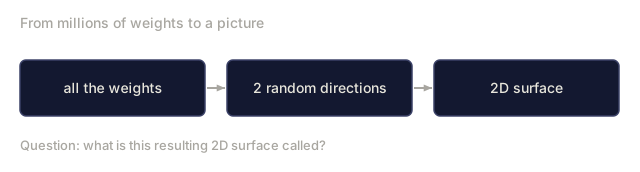
The loss is a function of all weights. For a model with 1 million weights, the loss landscape lives in 1,000,001-dimensional space. We visualize it by picking two random directions in weight space and plotting the loss along those directions, producing a 2D surface.

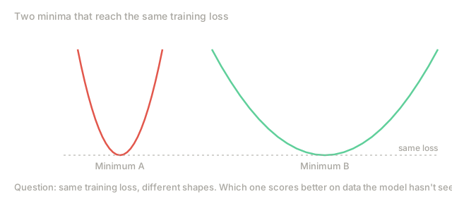
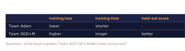
Sharp minima generalize poorly. Flat minima generalize well. This is one reason SGD with momentum often outperforms Adam on final test accuracy: its noise prevents settling into sharp minima.


Build It
Step 1: Define a test function
The Rosenbrock function is a classic optimization benchmark. Its minimum is at (1, 1) inside a narrow curved valley that is easy to find but hard to follow.
f(x, y) = (1 - x)^2 + 100 * (y - x^2)^2
def rosenbrock(params):
    x, y = params
    return (1 - x) ** 2 + 100 * (y - x ** 2) ** 2

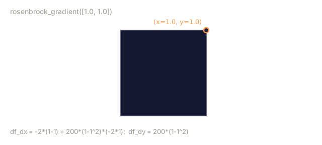
def rosenbrock_gradient(params):
    x, y = params
    df_dx = -2 * (1 - x) + 200 * (y - x ** 2) * (-2 * x)
    df_dy = 200 * (y - x ** 2)
    return [df_dx, df_dy]
Step 2: Vanilla gradient descent
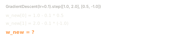
class GradientDescent:
    def __init__(self, lr=0.001):
        self.lr = lr

    def step(self, params, grads):
        return [p - self.lr * g for p, g in zip(params, grads)]
Step 3: SGD with momentum
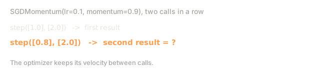
class SGDMomentum:
    def __init__(self, lr=0.001, momentum=0.9):
        self.lr = lr
        self.momentum = momentum
        self.velocity = None

    def step(self, params, grads):
        if self.velocity is None:
            self.velocity = [0.0] * len(params)
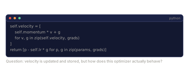
        self.velocity = [
            self.momentum * v + g
            for v, g in zip(self.velocity, grads)
        ]
        return [p - self.lr * v for p, v in zip(params, self.velocity)]
Step 4: Adam
class Adam:
    def __init__(self, lr=0.001, beta1=0.9, beta2=0.999, epsilon=1e-8):
        self.lr = lr
        self.beta1 = beta1
        self.beta2 = beta2
        self.epsilon = epsilon
        self.m = None
        self.v = None
        self.t = 0

    def step(self, params, grads):
        if self.m is None:
            self.m = [0.0] * len(params)
            self.v = [0.0] * len(params)

        self.t += 1

        self.m = [
            self.beta1 * m + (1 - self.beta1) * g
            for m, g in zip(self.m, grads)
        ]
        self.v = [
            self.beta2 * v + (1 - self.beta2) * g ** 2
            for v, g in zip(self.v, grads)
        ]

        m_hat = [m / (1 - self.beta1 ** self.t) for m in self.m]
        v_hat = [v / (1 - self.beta2 ** self.t) for v in self.v]

        return [
            p - self.lr * mh / (vh ** 0.5 + self.epsilon)
            for p, mh, vh in zip(params, m_hat, v_hat)
        ]
Step 5: Run and compare
def optimize(optimizer, func, grad_func, start, steps=5000):
    params = list(start)
    history = [params[:]]
    for _ in range(steps):
        grads = grad_func(params)
        params = optimizer.step(params, grads)
        history.append(params[:])
    return history

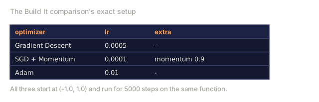
start = [-1.0, 1.0]

gd_history = optimize(GradientDescent(lr=0.0005), rosenbrock, rosenbrock_gradient, start)
sgd_history = optimize(SGDMomentum(lr=0.0001, momentum=0.9), rosenbrock, rosenbrock_gradient, start)
adam_history = optimize(Adam(lr=0.01), rosenbrock, rosenbrock_gradient, start)

for name, history in [("GD", gd_history), ("SGD+M", sgd_history), ("Adam", adam_history)]:
    final = history[-1]
    loss = rosenbrock(final)
    print(f"{name:6s} -> x={final[0]:.6f}, y={final[1]:.6f}, loss={loss:.8f}")
Expected output: Adam converges fastest. SGD with momentum follows a smoother path. Vanilla GD makes slow progress along the narrow valley.

Use It
In practice, you won't hand-roll any of this. Use PyTorch or JAX optimizers: they handle parameter groups, weight decay, gradient clipping, and GPU acceleration for you.
import torch

model = torch.nn.Linear(784, 10)

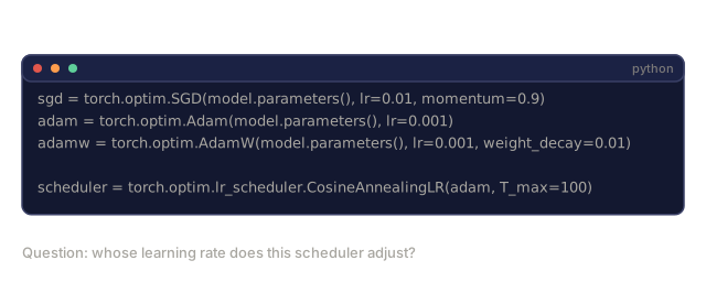
sgd = torch.optim.SGD(model.parameters(), lr=0.01, momentum=0.9)
adam = torch.optim.Adam(model.parameters(), lr=0.001)
adamw = torch.optim.AdamW(model.parameters(), lr=0.001, weight_decay=0.01)

scheduler = torch.optim.lr_scheduler.CosineAnnealingLR(adam, T_max=100)
Rules of thumb:
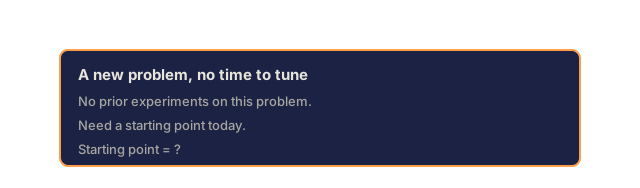
- Start with Adam (lr=0.001). It works for most problems without tuning.
- Switch to SGD with momentum (lr=0.01, momentum=0.9) when you need the best final accuracy and can afford more tuning.
- Use AdamW (Adam with decoupled weight decay) for transformers.
- Always use a learning rate schedule for training runs longer than a few epochs.
- If training is unstable, reduce the learning rate. If training is too slow, increase it.
Ship It
outputs/prompt-optimizer-guide.md walks you through choosing the right optimizer for whatever problem you're actually facing, instead of defaulting to Adam out of habit.
The optimizer classes you just built reappear in Phase 3, when we train a neural network from scratch.
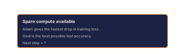
Here's the part that trips people up in practice: Adam winning your training curve doesn't mean Adam wins your model. It converges faster because it's aggressive about scaling each weight's step, and that same aggressiveness is what steers it into sharp, narrow minima. SGD with momentum crawls there slower, but the noise it carries along the way keeps knocking it out of the narrow ones, so it tends to land somewhere flatter and more forgiving on data it hasn't seen. If you're optimizing for a leaderboard number and have the compute to spare, don't assume Adam's faster loss curve means a better model. Run SGD with momentum as a second pass and compare test accuracy, not training speed.
Exercises
-
Learning rate sweep. Run vanilla gradient descent on the Rosenbrock function with learning rates [0.0001, 0.0005, 0.001, 0.005, 0.01]. Plot or print the final loss after 5000 steps for each. Find the largest learning rate that still converges.
-
Momentum comparison. Run SGD with momentum values [0.0, 0.5, 0.9, 0.99] on the Rosenbrock function. Track the loss at every step. Which momentum value converges fastest? Which overshoots?
-
Saddle point escape. Define the function
f(x, y) = x^2 - y^2(a saddle point at the origin). Start at (0.01, 0.01). Compare how vanilla GD, SGD with momentum, and Adam behave. Which escapes the saddle point? -
Implement learning rate decay. Add an exponential decay schedule to the GradientDescent class:
lr = lr_0 * 0.999^step. Compare convergence with and without decay on the Rosenbrock function.
Key Terms
| Term | What people say | What it actually means |
|---|---|---|
| Gradient descent | "Go downhill" | Update weights by subtracting the gradient scaled by the learning rate. The most basic optimizer. |
| Learning rate | "Step size" | A scalar that controls how far each update moves the weights. Too large causes divergence. Too small wastes compute. |
| Momentum | "Keep rolling" | Accumulate past gradients into a velocity vector. Dampens oscillations and accelerates movement through consistent directions. |
| SGD | "Random sampling" | Stochastic gradient descent. Compute gradient on a random subset instead of the full dataset. Almost always means mini-batch SGD in practice. |
| Mini-batch | "A chunk of data" | A small subset of training data (32-256 samples) used to estimate the gradient. Balances speed and gradient accuracy. |
| Adam | "The default optimizer" | Adaptive Moment Estimation. Tracks per-weight running averages of gradients and squared gradients to give each weight its own learning rate. |
| Bias correction | "Fix the cold start" | Adam's first and second moments are initialized to zero. Bias correction divides by (1 - beta^t) to compensate during early steps. |
| Learning rate schedule | "Change lr over time" | A function that adjusts the learning rate during training. Large steps early, small steps late. |
| Convex function | "One valley" | A function where any local minimum is the global minimum. Gradient descent always finds it. Neural network losses are not convex. |
| Saddle point | "Flat but not a minimum" | A point where the gradient is zero but it is a minimum in some directions and a maximum in others. Common in high dimensions. |
| Loss landscape | "The terrain" | The loss function plotted over weight space. Visualized by slicing along two random directions. |
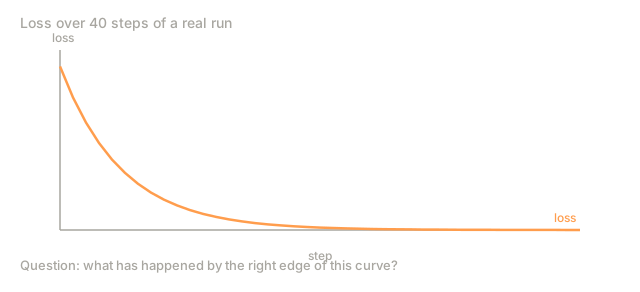
| Convergence | "Getting there" | The optimizer has reached a point where further steps do not meaningfully reduce the loss. |
Further Reading
- Sebastian Ruder: An overview of gradient descent optimization algorithms - comprehensive survey of all major optimizers
- Why Momentum Really Works (Distill) - interactive visualization of momentum dynamics
- Adam: A Method for Stochastic Optimization (Kingma & Ba, 2014) - the original Adam paper, readable and short
- Visualizing the Loss Landscape of Neural Nets (Li et al., 2018) - the paper that showed sharp vs flat minima
Code
- main.jl (text, 303 lines)
- optimizers.py (python, 288 lines)