Convex Optimization
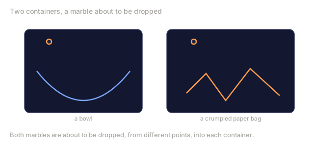
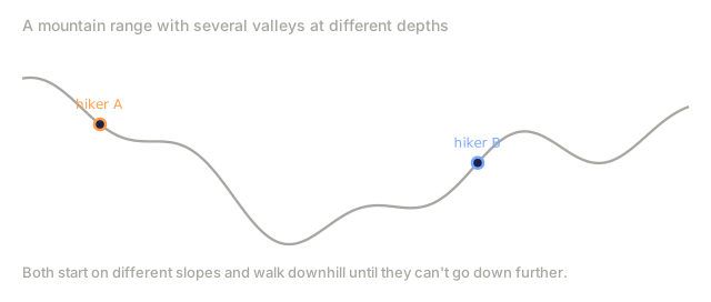
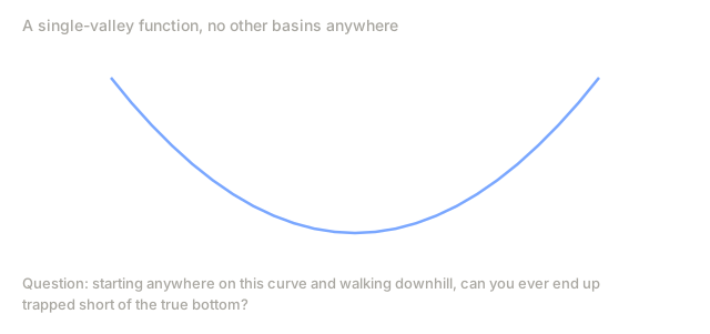
Convex problems have exactly one valley: walk downhill and you reach the bottom, guaranteed. Neural networks have millions of valleys and no such promise. Know which one you're standing in before you pick an optimizer.
Learning Objectives
- Test whether a function is convex using the definition, second derivative, and Hessian criteria
- Implement Newton's method and compare its quadratic convergence against gradient descent
- Solve constrained optimization problems using Lagrange multipliers and interpret KKT conditions
- Explain why neural network loss landscapes are non-convex yet SGD still finds good solutions
The Problem
Lesson 08 gave you gradient descent, momentum, and Adam: optimizers that walk downhill on any surface with no guarantees about where they end up. On a non-convex landscape, gradient descent can land in a bad local minimum, stall on a saddle point, or oscillate forever. You used it anyway, because neural networks are non-convex and there is no alternative.
Plenty of problems in machine learning aren't like that, though. Linear regression, logistic regression, SVMs, LASSO, ridge regression: all convex. For these, something stronger than walking downhill and hoping exists: optimization with mathematical guarantees. A convex problem has exactly one valley, so any algorithm that walks downhill reaches the global minimum. No restarts needed, no learning rate schedules, no prayer.
Convexity earns its keep in three ways. It tells you upfront whether a problem is easy (convex) or hard (non-convex). It hands you faster tools, like Newton's method, whose guarantees only hold in the easy case. And it explains ideas that show up throughout ML even outside pure convex problems: regularization as a constraint, duality in SVMs, and why deep learning still works despite breaking every nice property convexity would have given it.
The Concept
Convex sets
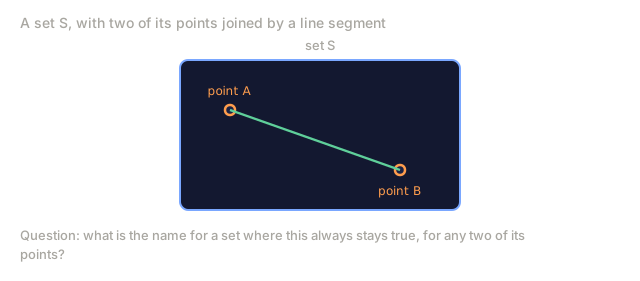
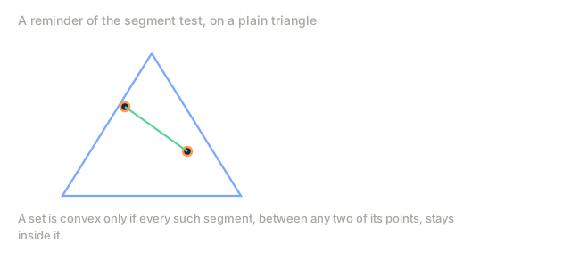
A set S is convex if for any two points in S, the line segment between them also lies entirely in S.
| Convex sets | Not convex |
|---|---|
| Rectangle: any two points inside can be connected by a line segment that stays inside | Star/crescent shape: a line between two interior points can pass outside the set |
| Triangle: same property holds for all interior points | Donut/annulus: the hole means some line segments leave the set |
| The line segment between any two points stays within the set | The line segment between some pairs of points exits the set |
Formal test: for any points x, y in S and any t in [0, 1], the point tx + (1-t)y is also in S.
Examples of convex sets:
- A line, a plane, all of R^n
- A ball (circle, sphere, hypersphere)
- A halfspace: {x : a^T x <= b}
- The intersection of any number of convex sets
Examples of non-convex sets:
- A donut (annulus)
- The union of two disjoint circles
- Any set with a "dent" or "hole"
Convex functions
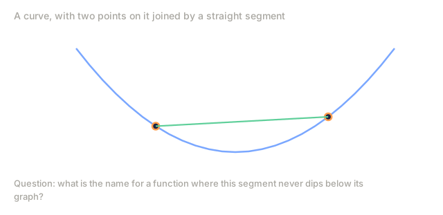
A function f is convex if its domain is a convex set and for any two points x, y in its domain and any t in [0, 1]:
f(tx + (1-t)y) <= t*f(x) + (1-t)*f(y)
Geometrically: the line segment between any two points on the graph lies above or on the graph.
| Property | Convex function | Non-convex function |
|---|---|---|
| Line segment test | The line between any two points on the graph lies above or on the curve | The line between some points on the graph dips below the curve |
| Shape | Single bowl/valley curving upward | Multiple peaks and valleys with mixed curvature |
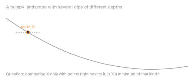
| Local minima | Every local minimum is the global minimum | Multiple local minima may exist at different heights |
Common convex functions:
- f(x) = x^2 (parabola)
- f(x) = |x| (absolute value)
- f(x) = e^x (exponential)
- f(x) = max(0, x) (ReLU, though piecewise linear)
- f(x) = -log(x) for x > 0 (negative log)
- Any linear function f(x) = a^T x + b (both convex and concave)
Testing for convexity
Three practical tests, from easiest to most rigorous.
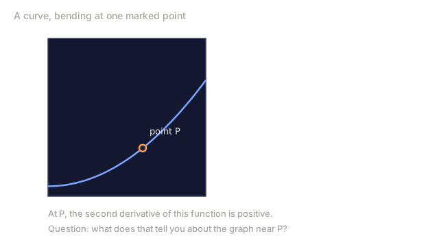
Test 1: Second derivative test (1D). If f''(x) >= 0 for all x, then f is convex.
- f(x) = x^2: f''(x) = 2 >= 0. Convex.
- f(x) = x^3: f''(x) = 6x. Negative for x < 0. Not convex.
- f(x) = e^x: f''(x) = e^x > 0. Convex.
Test 2: Hessian test (multivariate). If the Hessian matrix H(x) is positive semidefinite for all x, then f is convex. The Hessian is the matrix of second partial derivatives.
Test 3: Definition test. Check the inequality f(tx + (1-t)y) <= t*f(x) + (1-t)*f(y) directly. Useful for functions where derivatives are hard to compute.
Why convexity matters
The central theorem of convex optimization:
For a convex function, every local minimum is a global minimum.
This means gradient descent cannot get trapped. Any downhill path leads to the same answer. The algorithm is guaranteed to converge to the optimal solution.

Consequences:
- No need for random restarts
- No need for sophisticated learning rate schedules
- Convergence proofs are possible (rate depends on function properties)
- The solution is unique (up to flat regions)
Convex vs non-convex in ML
| Problem | Convex? | Why |
|---|---|---|
| Linear regression (MSE) | Yes | Loss is quadratic in weights |
| Logistic regression | Yes | Log-loss is convex in weights |
| SVM (hinge loss) | Yes | Maximum of linear functions |
| LASSO (L1 regression) | Yes | Sum of convex functions is convex |
| Ridge regression (L2) | Yes | Quadratic + quadratic = convex |
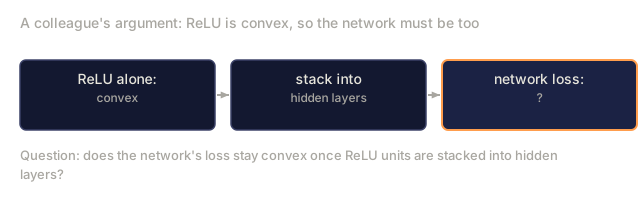
| Neural network (any loss) | No | Nonlinear activations create non-convex landscape |
| k-means clustering | No | Discrete assignment step |
| Matrix factorization | No | Product of unknowns |
Linear models with convex losses are convex. The moment you add hidden layers with nonlinear activations, convexity breaks.
The Hessian matrix
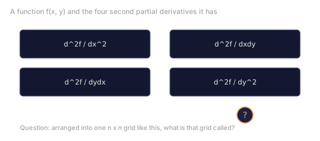
The Hessian H of a function f: R^n -> R is the n x n matrix of second partial derivatives.
H[i][j] = d^2 f / (dx_i dx_j)
For f(x, y) = x^2 + 3xy + y^2:
df/dx = 2x + 3y       d^2f/dx^2 = 2      d^2f/dxdy = 3
df/dy = 3x + 2y       d^2f/dydx = 3      d^2f/dy^2 = 2

H = [ 2  3 ]
    [ 3  2 ]
The Hessian tells you about curvature:
- Eigenvalues all positive: the function curves upward in every direction (convex at that point)
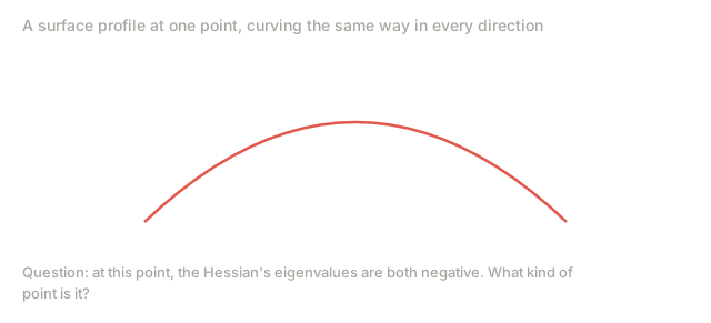
- Eigenvalues all negative: curves downward in every direction (concave, a local max)
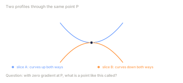
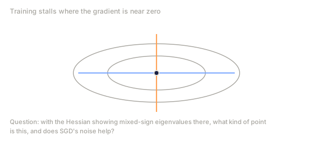
- Mixed signs: saddle point (curves up in some directions, down in others)
- Zero eigenvalue: flat in that direction (degenerate)
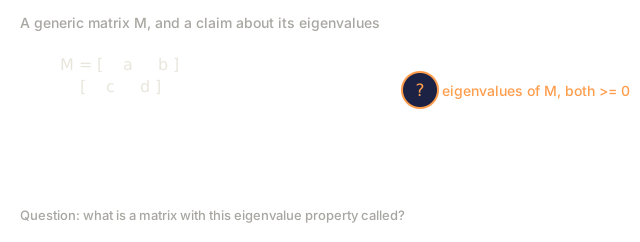
For convexity, the Hessian must be positive semidefinite (all eigenvalues >= 0) everywhere, not just at one point.
Newton's method
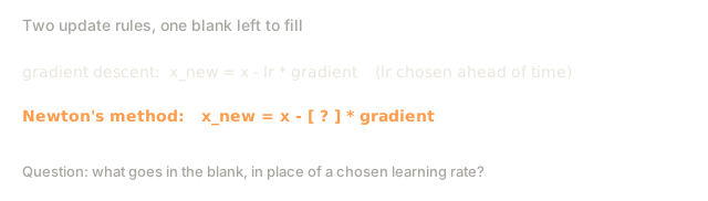
Gradient descent uses first-order information: the gradient. Newton's method goes a step further and uses second-order information, the Hessian, fitting a quadratic approximation at the current point and jumping straight to that quadratic's minimum.
Update rule:
  x_new = x - H^(-1) * gradient

Compare to gradient descent:
  x_new = x - lr * gradient
Newton's method replaces the scalar learning rate with the inverse Hessian. This automatically adjusts the step size and direction based on local curvature.

Advantages:
- Quadratic convergence near the minimum (error squares each step)
- No learning rate to tune
- Scale-invariant (works regardless of how you parameterize the problem)
Disadvantages:
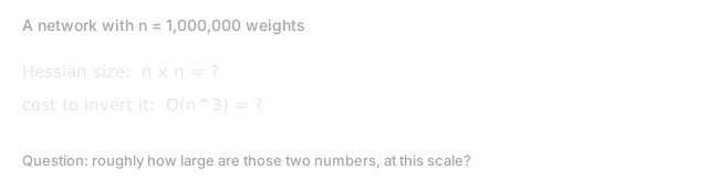
- Computing the Hessian costs O(n^2) memory and O(n^3) to invert
- For a neural network with 1 million weights, that is 10^12 entries and 10^18 operations
- Not practical for deep learning
Constrained optimization
Unconstrained optimization: minimize f(x) over all x. Constrained optimization: minimize f(x) subject to constraints.
Real problems have constraints. You want to minimize cost but your budget is limited. You want to minimize error but your model complexity is bounded.

Lagrange multipliers
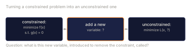
The method of Lagrange multipliers converts a constrained problem into an unconstrained one.
Problem: minimize f(x) subject to g(x) = 0.
Solution: introduce a new variable (the Lagrange multiplier lambda) and solve the unconstrained problem:
L(x, lambda) = f(x) + lambda * g(x)
At the solution, the gradient of L is zero:
dL/dx = df/dx + lambda * dg/dx = 0
dL/dlambda = g(x) = 0
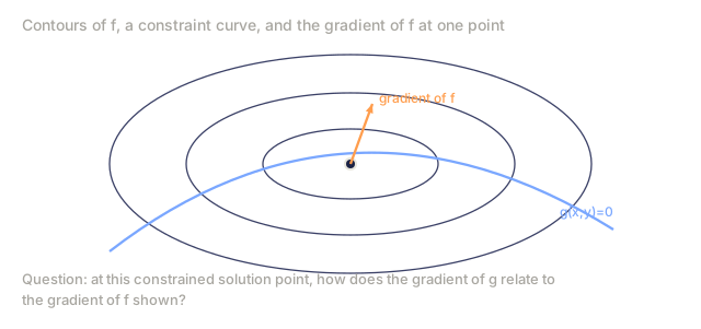
Geometric intuition: at the constrained minimum, the gradient of f must be parallel to the gradient of the constraint g. If they were not parallel, you could move along the constraint surface and reduce f further.

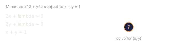
Example: minimize f(x,y) = x^2 + y^2 subject to x + y = 1.
L = x^2 + y^2 + lambda(x + y - 1)

dL/dx = 2x + lambda = 0  =>  x = -lambda/2
dL/dy = 2y + lambda = 0  =>  y = -lambda/2
dL/dlambda = x + y - 1 = 0

From first two: x = y
Substituting: 2x = 1, so x = y = 0.5, lambda = -1
The closest point on the line x + y = 1 to the origin is (0.5, 0.5).
KKT conditions
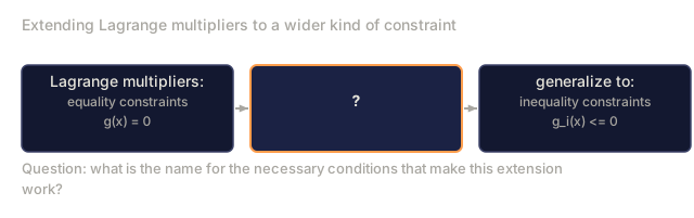
The Karush-Kuhn-Tucker conditions extend Lagrange multipliers to inequality constraints.
Problem: minimize f(x) subject to g_i(x) <= 0 for i = 1, ..., m.
The KKT conditions (necessary for optimality):
1. Stationarity:    df/dx + sum(lambda_i * dg_i/dx) = 0
2. Primal feasibility:  g_i(x) <= 0  for all i
3. Dual feasibility:    lambda_i >= 0  for all i
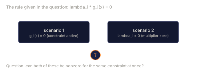
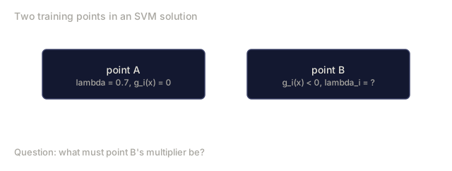
4. Complementary slackness:  lambda_i * g_i(x) = 0  for all i
Complementary slackness is the key insight: either the constraint is active (g_i = 0, the solution sits on the boundary) or the multiplier is zero (the constraint does not matter). A constraint that does not affect the solution has lambda = 0.
KKT conditions are central to SVMs. The support vectors are the data points where the constraint is active (lambda > 0). All other data points have lambda = 0 and do not affect the decision boundary.
Regularization as constrained optimization
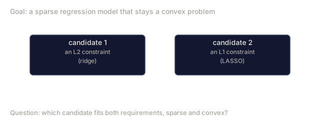
L1 and L2 regularization aren't arbitrary tricks: they're constrained optimization problems wearing a disguise.
L2 regularization (Ridge):
minimize  Loss(w)  subject to  ||w||^2 <= t

Equivalent unconstrained form:
minimize  Loss(w) + lambda * ||w||^2
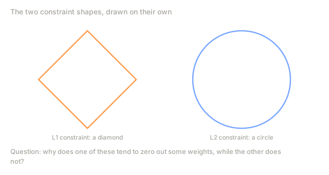
The constraint ||w||^2 <= t defines a ball (circle in 2D, sphere in 3D). The solution is where the loss contours first touch this ball.
L1 regularization (LASSO):
minimize  Loss(w)  subject to  ||w||_1 <= t

Equivalent unconstrained form:
minimize  Loss(w) + lambda * ||w||_1
The constraint ||w||_1 <= t defines a diamond (rotated square in 2D).
| Property | L2 constraint (circle) | L1 constraint (diamond) |
|---|---|---|
| Constraint shape | Circle (sphere in higher dims) | Diamond (rotated square in 2D) |
| Where loss contour touches | Smooth boundary — any point on the circle | Corner — aligned with an axis |
| Solution behavior | Weights are small but nonzero | Some weights are exactly zero (sparse) |
| Result | Weight shrinkage | Feature selection |
This explains why L1 produces sparse models (feature selection) while L2 only shrinks weights. The diamond has corners aligned with axes. Loss contours are more likely to touch a corner, setting one or more weights exactly to zero.
Duality
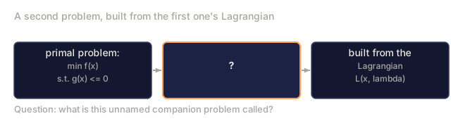
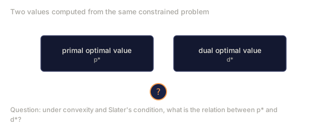
Every constrained optimization problem (the primal) has a companion problem (the dual). For convex problems, the primal and dual have the same optimal value. This is strong duality.
The Lagrangian dual function:
Primal: minimize f(x) subject to g(x) <= 0
Lagrangian: L(x, lambda) = f(x) + lambda * g(x)
Dual function: d(lambda) = min_x L(x, lambda)
Dual problem: maximize d(lambda) subject to lambda >= 0
Why duality matters:
- The dual problem is sometimes easier to solve than the primal
- SVMs are solved in their dual form, where the problem depends on dot products between data points (enabling the kernel trick)
- The dual provides a lower bound on the primal optimum, useful for checking solution quality
For SVMs specifically:
Primal: find w, b that maximize the margin 2/||w|| subject to
        y_i(w^T x_i + b) >= 1 for all i

Dual:   maximize sum(alpha_i) - 0.5 * sum_ij(alpha_i * alpha_j * y_i * y_j * x_i^T x_j)
        subject to alpha_i >= 0 and sum(alpha_i * y_i) = 0

The dual only involves dot products x_i^T x_j.
Replace x_i^T x_j with K(x_i, x_j) to get the kernel trick.
Why deep learning works despite non-convexity
Neural network loss functions are wildly non-convex. By every classical measure, optimizing them should fail, yet stochastic gradient descent finds good solutions reliably.
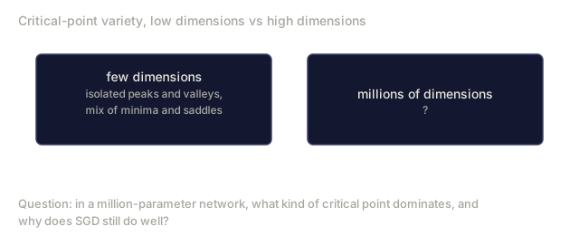
Most local minima are good enough. In high-dimensional spaces, random critical points (where the gradient is zero) are overwhelmingly saddle points, not local minima. The few local minima that exist tend to have loss values close to the global minimum. Getting trapped in a terrible local minimum is extremely unlikely when the parameter space has millions of dimensions.
Saddle points are the real obstacle, not local minima. In a function with n parameters, a saddle point has a mix of positive and negative curvature directions. For a random critical point in high dimensions, the probability of all n eigenvalues being positive (local minimum) is roughly 2^(-n). Almost all critical points are saddle points, and SGD's noise helps escape them.
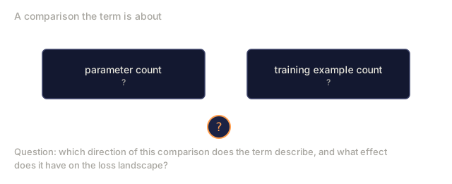
Overparameterization smooths the landscape. Networks with more parameters than training examples have smoother, more connected loss surfaces. Wider networks have fewer bad local minima. This is counterintuitive but empirically consistent.
Loss landscape structure:
| Property | Low-dimensional space | High-dimensional space |
|---|---|---|
| Landscape | Many isolated peaks and valleys | Smoothly connected valleys |
| Minima | Many isolated local minima | Few bad local minima; most are near-optimal |
| Navigation | Hard to find global minimum | Many paths lead to good solutions |
| Critical points | Mix of local minima and saddle points | Overwhelmingly saddle points, not local minima |
Stochastic noise acts as implicit regularization. Mini-batch SGD adds noise that prevents settling into sharp minima. Sharp minima overfit; flat minima generalize. The noise biases optimization toward flat regions of the loss landscape.
Second-order methods in practice
Pure Newton's method is impractical for large models. Several approximations make second-order information usable.
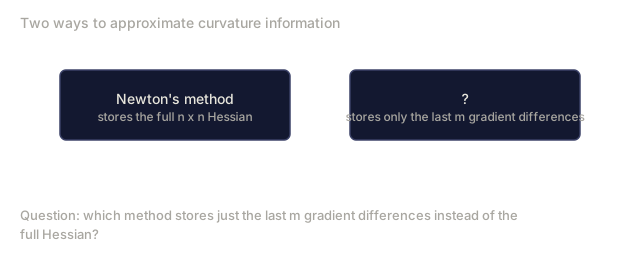
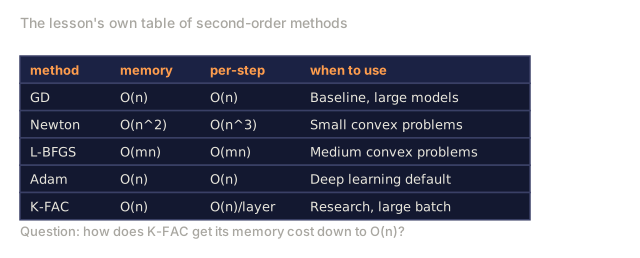
L-BFGS (Limited-memory BFGS): Approximates the inverse Hessian using the last m gradient differences. Requires O(mn) memory instead of O(n^2). Works well for problems with up to ~10,000 parameters. Used in classical ML (logistic regression, CRFs) but not deep learning.
Natural gradient: Uses the Fisher information matrix (expected Hessian of the log-likelihood) instead of the standard Hessian. This accounts for the geometry of probability distributions. K-FAC (Kronecker-Factored Approximate Curvature) approximates the Fisher matrix as a Kronecker product, making it practical for neural networks.
Hessian-free optimization: Uses conjugate gradient to solve Hx = g without ever forming H. Only requires Hessian-vector products, which can be computed in O(n) time via automatic differentiation.
Diagonal approximations: Adam's second moment is a diagonal approximation of the Hessian's diagonal. AdaHessian extends this by using actual Hessian diagonal elements via Hutchinson's estimator.
| Method | Memory | Per-step cost | When to use |
|---|---|---|---|
| Gradient descent | O(n) | O(n) | Baseline, large models |
| Newton's method | O(n^2) | O(n^3) | Small convex problems |
| L-BFGS | O(mn) | O(mn) | Medium convex problems |
| Adam | O(n) | O(n) | Deep learning default |
| K-FAC | O(n) | O(n) per layer | Research, large-batch training |





Build It
Step 1: Convexity checker
Build a function that tests convexity empirically by sampling points and checking the definition.
import random
import math

def check_convexity(f, dim, bounds=(-5, 5), samples=1000):
    violations = 0
    for _ in range(samples):
        x = [random.uniform(*bounds) for _ in range(dim)]
        y = [random.uniform(*bounds) for _ in range(dim)]
        t = random.uniform(0, 1)
        mid = [t * xi + (1 - t) * yi for xi, yi in zip(x, y)]
        lhs = f(mid)
        rhs = t * f(x) + (1 - t) * f(y)
        if lhs > rhs + 1e-10:
            violations += 1
    return violations == 0, violations
Step 2: Newton's method for 2D
Implement Newton's method using an explicit Hessian. Compare convergence speed against gradient descent.
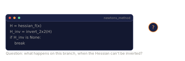
def newtons_method(f, grad_f, hessian_f, x0, steps=50, tol=1e-12):
    x = list(x0)
    history = [x[:]]
    for _ in range(steps):
        g = grad_f(x)
        H = hessian_f(x)
        det = H[0][0] * H[1][1] - H[0][1] * H[1][0]
        if abs(det) < 1e-15:
            break
        H_inv = [
            [H[1][1] / det, -H[0][1] / det],
            [-H[1][0] / det, H[0][0] / det],
        ]
        dx = [
            H_inv[0][0] * g[0] + H_inv[0][1] * g[1],
            H_inv[1][0] * g[0] + H_inv[1][1] * g[1],
        ]
        x = [x[0] - dx[0], x[1] - dx[1]]
        history.append(x[:])
        if sum(gi ** 2 for gi in g) < tol:
            break
    return history
Step 3: Lagrange multiplier solver
Solve constrained optimization using gradient descent on the Lagrangian.
def lagrange_solve(f_grad, g_val, g_grad, x0, lr=0.01,
                   lr_lambda=0.01, steps=5000):
    x = list(x0)
    lam = 0.0
    history = []
    for _ in range(steps):
        fg = f_grad(x)
        gv = g_val(x)
        gg = g_grad(x)
        x = [
            xi - lr * (fgi + lam * ggi)
            for xi, fgi, ggi in zip(x, fg, gg)
        ]
        lam = lam + lr_lambda * gv
        history.append((x[:], lam, gv))
    return history
Step 4: Compare first-order vs second-order
Run gradient descent and Newton's method on the same quadratic function. Count the steps to convergence.
def quadratic(x):
    return 5 * x[0] ** 2 + x[1] ** 2

def quadratic_grad(x):
    return [10 * x[0], 2 * x[1]]

def quadratic_hessian(x):
    return [[10, 0], [0, 2]]
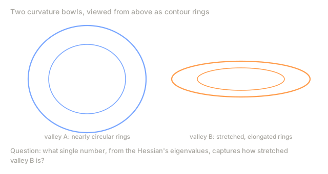
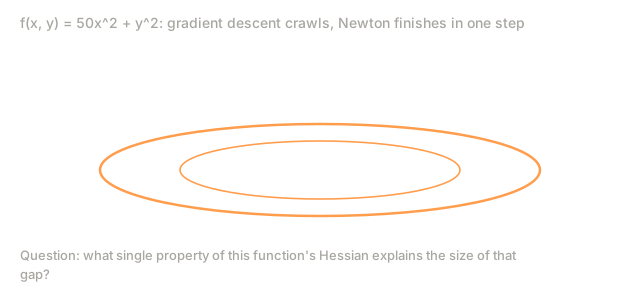
Newton's method will converge in 1 step (it is exact for quadratics). Gradient descent will take hundreds of steps because the eigenvalues of the Hessian differ by a factor of 5, creating an elongated valley.



Use It
Convexity analysis applies directly when choosing ML models and solvers.
For convex problems (logistic regression, SVMs, LASSO):
- Use dedicated solvers (liblinear, CVXPY, scipy.optimize.minimize with method='L-BFGS-B')
- Expect a unique global solution
- Second-order methods are practical and fast
For non-convex problems (neural networks):
- Use first-order methods (SGD, Adam)
- Accept that the solution depends on initialization and randomness
- Use overparameterization, noise, and learning rate schedules as implicit regularization
- Do not waste time searching for the global minimum. A good local minimum is sufficient.
from scipy.optimize import minimize

result = minimize(
    fun=lambda w: sum((y - X @ w) ** 2) + 0.1 * sum(w ** 2),
    x0=np.zeros(d),
    method='L-BFGS-B',
    jac=lambda w: -2 * X.T @ (y - X @ w) + 0.2 * w,
)
For SVMs, the dual formulation lets you use the kernel trick:
from sklearn.svm import SVC

svm = SVC(kernel='rbf', C=1.0)
svm.fit(X_train, y_train)
print(f"Support vectors: {svm.n_support_}")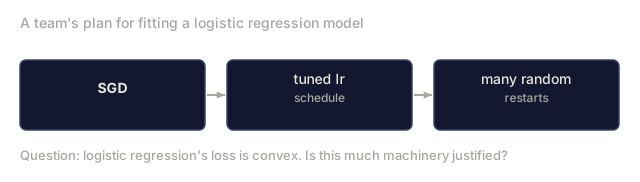
Ship It
This lesson produces:
code/convex.py, with from-scratch implementations of the convexity checker, Newton's method, the Lagrange multiplier solver, and the Hessian eigenvalue analysis this lesson walks throughoutputs/skill-convexity-checker.md, a skill that determines whether a given optimization problem is convex and points you to the right solver once you know
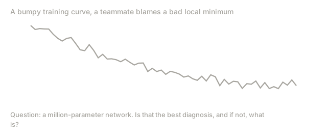
The mistake I see most often is treating a bumpy loss curve as a diagnosis instead of a symptom. In a million-parameter network, a rough training run is far more likely to be a bad learning rate, a gradient issue, or a data problem than an actual bad local minimum. Non-convex doesn't mean cursed. It means the guarantees are gone, so you have to go look at what actually broke instead of assuming the landscape is out to get you.
The flip side matters just as much. If you do have a convex problem on your hands, a logistic regression, an SVM, a LASSO fit, stop babysitting a learning rate schedule like it's a transformer. Reach for a real solver, get the exact answer, and spend your debugging time somewhere it will actually pay off.
Exercises
-
Convexity gallery. Test these functions for convexity using the checker: f(x) = x^4, f(x) = sin(x), f(x,y) = x^2 + y^2, f(x,y) = x*y, f(x) = max(x, 0). Explain why each result makes sense.
-
Newton vs gradient descent race. Run both methods on f(x,y) = 50*x^2 + y^2 from the starting point (10, 10). How many steps does each need to reach loss < 1e-10? What happens to gradient descent when the condition number (ratio of largest to smallest Hessian eigenvalue) increases?
-
Lagrange multiplier geometry. Minimize f(x,y) = (x-3)^2 + (y-3)^2 subject to x + 2y = 4. Verify the solution by checking that the gradient of f is parallel to the gradient of g at the solution.
-
Regularization constraint. Implement L1-constrained optimization: minimize (x-3)^2 + (y-2)^2 subject to |x| + |y| <= 1. Show that the solution has one coordinate equal to zero (sparsity from the diamond constraint).
-
Hessian eigenvalue analysis. Compute the Hessian of the Rosenbrock function (the curved-valley benchmark from Lesson 08) at (1,1) and at (-1,1). Compute eigenvalues at both points. What do the eigenvalues tell you about the curvature at the minimum versus far from it?
Key Terms
| Term | What it means |
|---|---|
| Convex set | A set where the line segment between any two points in the set stays inside the set |
| Convex function | A function where the line between any two points on its graph lies above or on the graph. Equivalently, Hessian is positive semidefinite everywhere |
| Local minimum | A point lower than all nearby points. For convex functions, every local minimum is the global minimum |
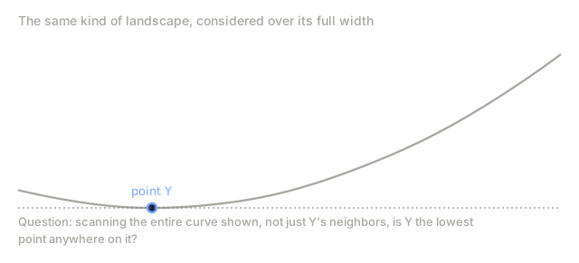
| Global minimum | The lowest point of a function over its entire domain |
| Hessian matrix | The matrix of all second partial derivatives. Encodes curvature information |
| Positive semidefinite | A matrix whose eigenvalues are all non-negative. The multidimensional analogue of "second derivative >= 0" |
| Condition number | Ratio of largest to smallest eigenvalue of the Hessian. High condition number means elongated valleys and slow gradient descent |
| Newton's method | Second-order optimizer that uses the inverse Hessian to determine step direction and size. Quadratic convergence near the minimum |
| Lagrange multiplier | A variable introduced to convert a constrained optimization problem into an unconstrained one |
| KKT conditions | Necessary conditions for optimality with inequality constraints. Generalize Lagrange multipliers |
| Complementary slackness | At the solution, either a constraint is active or its multiplier is zero. Never both nonzero |
| Duality | Every constrained problem has a companion dual problem. For convex problems, both have the same optimal value |
| Strong duality | Primal and dual optimal values are equal. Holds for convex problems satisfying Slater's condition |
| L-BFGS | Approximate second-order method that stores the last m gradient differences instead of the full Hessian |
| Saddle point | A point where the gradient is zero but it is a minimum in some directions and a maximum in others |
| Overparameterization | Using more parameters than training examples. Smooths the loss landscape and reduces bad local minima |
Further Reading
- Boyd & Vandenberghe: Convex Optimization - the standard textbook, freely available online
- Bottou, Curtis, Nocedal: Optimization Methods for Large-Scale Machine Learning (2018) - bridges convex optimization theory and deep learning practice
- Choromanska et al.: The Loss Surfaces of Multilayer Networks (2015) - why non-convex neural network landscapes are not as bad as they seem
- Nocedal & Wright: Numerical Optimization - comprehensive reference for Newton's method, L-BFGS, and constrained optimization
Code
- convex.py (python, 636 lines)