Naive Bayes
The "naive" assumption is wrong, and it works anyway. That's the beauty of it.
Learning Objectives
- Implement Multinomial Naive Bayes from scratch with Laplace smoothing for text classification
- Explain why the naive independence assumption is mathematically wrong but produces correct class rankings in practice
- Compare Multinomial, Bernoulli, and Gaussian Naive Bayes variants and select the right one for a given feature type
- Evaluate Naive Bayes against logistic regression on high-dimensional sparse data and explain the bias-variance tradeoff at work
The Problem
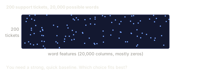
You need to classify text. Emails into spam or not-spam. Customer reviews into positive or negative. Support tickets into categories. You have thousands of features (one per word) and limited training data.
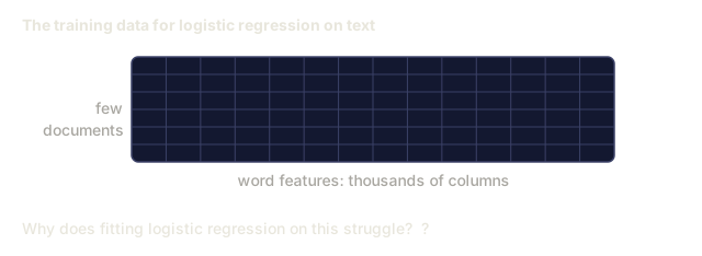
Most classifiers choke here. Logistic regression needs enough samples to estimate thousands of weights reliably. Decision trees split on one word at a time and overfit wildly. KNN in 10,000 dimensions is meaningless because every point is equally far from every other point.
Naive Bayes handles this. It makes a mathematically wrong assumption (that every feature is independent of every other feature given the class), and it still outperforms "smarter" models on text classification, especially with small training sets. It trains in a single pass through the data. It scales to millions of features. It produces probability estimates (though often poorly calibrated due to the independence assumption).
Understanding why a wrong assumption leads to good predictions teaches a fundamental lesson about machine learning: winning is about the bias-variance tradeoff for your data, not about which model's assumptions are most accurate.
The Concept
Bayes' Theorem (Quick Review)
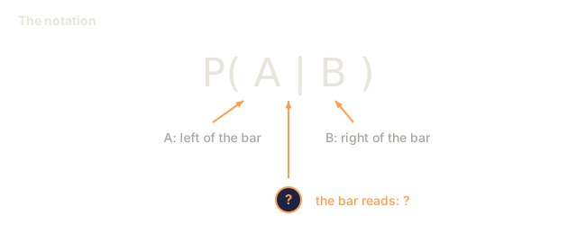
Bayes' theorem flips conditional probabilities:
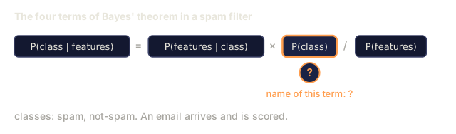
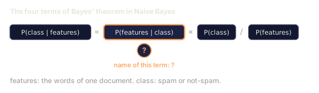
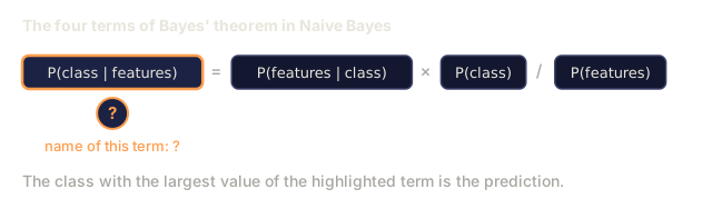
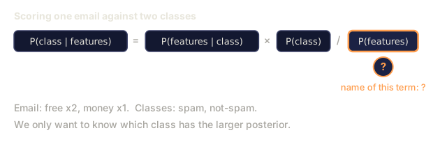
P(class | features) = P(features | class) * P(class) / P(features)
We want P(class | features): the probability that a document belongs to a class, given the words in it. We get there from three pieces:
P(features | class): the likelihood of seeing these words in documents of this classP(class): the prior probability of the class (how common is spam in general?)P(features): the evidence. It's the same for every class, so we can ignore it when comparing them.
The class with the highest P(class | features) wins.
The Naive Independence Assumption
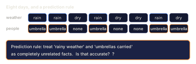
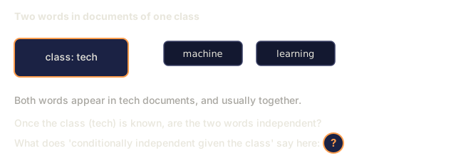
The naive assumption: every feature is conditionally independent of every other feature, given the class.
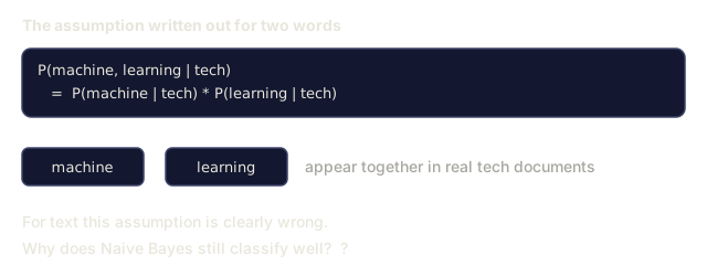
P(w1, w2, ..., wn | class) = P(w1 | class) * P(w2 | class) * ... * P(wn | class)
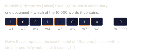
Why settle for something this blunt? Because the alternative is intractable. Computing P(features | class) exactly means estimating the joint probability of all features together, and with a vocabulary of 10,000 words that's a distribution over 2^10,000 possible combinations. Impossible. The naive assumption trades that one impossible joint distribution for n simple per-feature distributions, each of which needs only a count.
This assumption is obviously wrong. The words "machine" and "learning" are not independent in any document. But classification only cares about rankings: which class scores highest. Correct probability estimates were never the point. The independence assumption introduces systematic errors, but those errors hit all classes about equally, so the ranking survives.
Why It Still Works
Three reasons:
-
Ranking beats calibration. Classification only needs the top-ranked class to be correct. Even if P(spam) = 0.99999 when the true probability is 0.7, the classifier still picks spam. Winning the ranking is the job; getting the exact probability right never was.
-
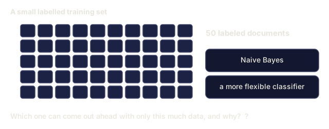
High bias, low variance. The independence assumption is a strong prior. It constrains the model heavily, which prevents overfitting. With limited training data, a model that's slightly wrong but stable beats a model that's theoretically right but wildly unstable. This is the bias-variance tradeoff in action.
-
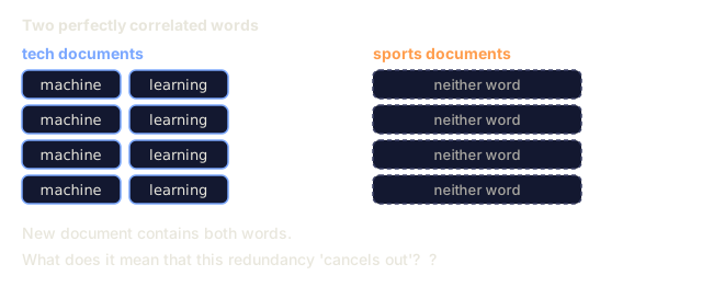
Feature redundancy cancels out. Correlated features provide redundant evidence. The classifier double-counts this evidence, but it double-counts it for the correct class too. If "machine" and "learning" always appear together, both provide evidence for the "tech" class. NB counts them twice, but it counts them twice for the right class.
A fourth, practical reason: Naive Bayes is extremely fast. Training is a single pass through the data counting frequencies. Prediction is a matrix multiplication. You can train on a million documents in seconds, which means you can iterate faster, try more feature sets, and run more experiments than with slower models.
The Math Step by Step
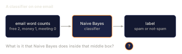
Let's trace through a concrete example. Suppose we have two classes: spam and not-spam. Our vocabulary has three words: "free", "money", "meeting".
Training data:
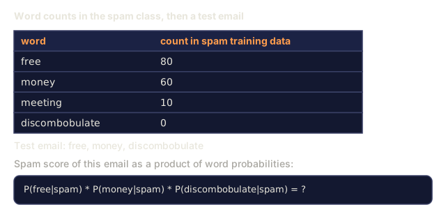
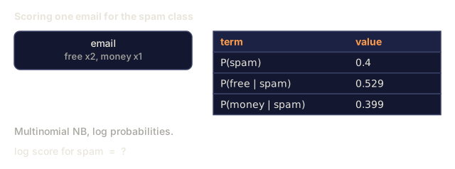
- Spam emails mention "free" 80 times, "money" 60 times, "meeting" 10 times (150 total words)
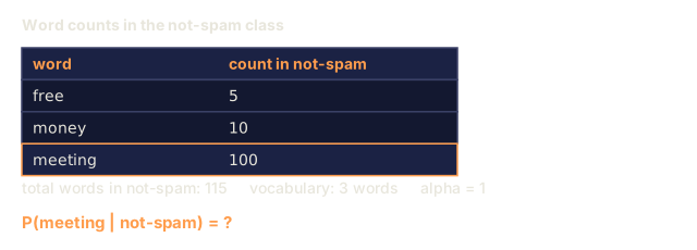
- Not-spam emails mention "free" 5 times, "money" 10 times, "meeting" 100 times (115 total words)
- 40% of emails are spam, 60% are not-spam
With Laplace smoothing (alpha=1):
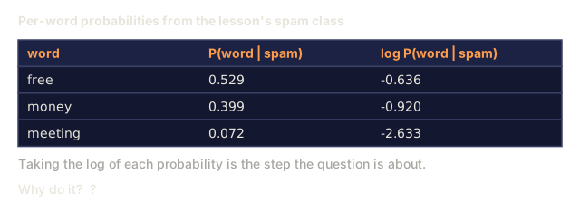
P(free | spam)    = (80 + 1) / (150 + 3) = 81/153 = 0.529
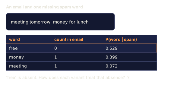
P(money | spam)   = (60 + 1) / (150 + 3) = 61/153 = 0.399
P(meeting | spam) = (10 + 1) / (150 + 3) = 11/153 = 0.072

P(free | not-spam)    = (5 + 1) / (115 + 3) = 6/118 = 0.051
P(money | not-spam)   = (10 + 1) / (115 + 3) = 11/118 = 0.093
P(meeting | not-spam) = (100 + 1) / (115 + 3) = 101/118 = 0.856
New email contains: "free" (2 times), "money" (1 time), "meeting" (0 times).
log P(spam | email) = log(0.4) + 2*log(0.529) + 1*log(0.399) + 0*log(0.072)
                    = -0.916 + 2*(-0.637) + (-0.919) + 0
                    = -3.109

log P(not-spam | email) = log(0.6) + 2*log(0.051) + 1*log(0.093) + 0*log(0.856)
                        = -0.511 + 2*(-2.976) + (-2.375) + 0
                        = -8.838
Spam wins by a large margin. The word "free" appearing twice is strong evidence for spam. Note that "meeting" not appearing contributes zero to both log sums (0 * log(P)): in Multinomial NB, absent words have no effect. Bernoulli NB is the variant that explicitly models word absence.
Three Variants
Naive Bayes comes in three flavors. Each models P(feature | class) differently.
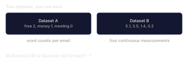
Multinomial Naive Bayes
Models each feature as a count. Best for text data where features are word frequencies or TF-IDF values.
P(word_i | class) = (count of word_i in class + alpha) / (total words in class + alpha * vocab_size)
The alpha is Laplace smoothing (explained below). This variant is the workhorse for text classification.
Gaussian Naive Bayes
Models each feature as a normal distribution. Best for continuous features.
P(x_i | class) = (1 / sqrt(2 * pi * var)) * exp(-(x_i - mean)^2 / (2 * var))
Each class gets its own mean and variance per feature. This works well when features genuinely follow a bell curve within each class.
Bernoulli Naive Bayes
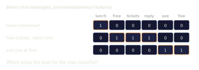
Models each feature as binary (present or absent). Best for short text or binary feature vectors.
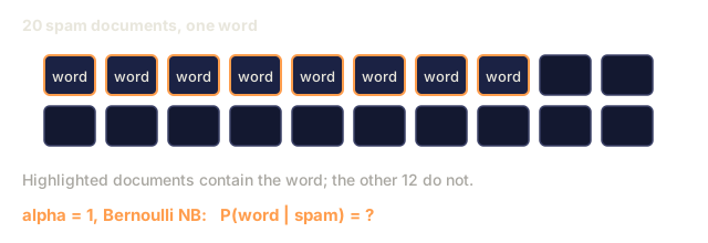
P(word_i | class) = (docs in class containing word_i + alpha) / (total docs in class + 2 * alpha)
Unlike Multinomial, Bernoulli explicitly penalizes the absence of a word. If "free" typically appears in spam but is absent from this email, Bernoulli counts that as evidence against spam.
When to Use Each Variant
| Variant | Feature Type | Best For | Example |
|---|---|---|---|
| Multinomial | Counts or frequencies | Text classification, bag-of-words | Email spam, topic classification |
| Gaussian | Continuous values | Tabular data with normal-ish features | Iris classification, sensor data |
| Bernoulli | Binary (0/1) | Short text, binary feature vectors | SMS spam, presence/absence features |
Laplace Smoothing
Laplace smoothing adds a small count alpha (usually 1) to every feature count, so a word that never showed up in training doesn't zero out the whole prediction:
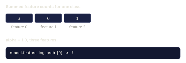
P(word_i | class) = (count(word_i, class) + alpha) / (total_words_in_class + alpha * vocab_size)
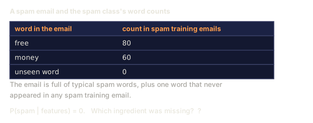
Here's why that matters. Without smoothing, P(word | class) = 0/N = 0 for any word that never appeared in a class's training data. One zero multiplied through the entire product makes P(class | features) = 0, regardless of all other evidence. A single unseen word destroys the entire prediction, no matter how much other evidence supports it.
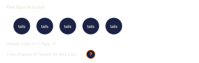
With alpha=1, every word gets at least a tiny probability. The word "discombobulate" appearing in a test email no longer kills the spam probability. The smoothing has a Bayesian interpretation: it's equivalent to placing a uniform Dirichlet prior on the word distributions.
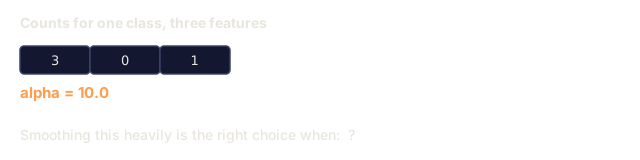
Higher alpha means stronger smoothing (more uniform distributions). Lower alpha means the model trusts the data more. Alpha is a hyperparameter you tune.
The effect of alpha:
| Alpha | Effect | When to use |
|---|---|---|
| 0.001 | Almost no smoothing, trust the data | Very large training set, no unseen features expected |
| 0.1 | Light smoothing | Large training set |
| 1.0 | Standard Laplace smoothing | Default starting point |
| 10.0 | Heavy smoothing, flattens distributions | Very small training set, many unseen features expected |
Log-Space Computation
Working in log space means replacing probability multiplication with addition of logarithms:
log P(class | features) = log P(class) + sum_i log P(feature_i | class)
The reason: multiplying hundreds of probabilities, each less than 1, causes floating-point underflow. The product becomes zero in floating point even though the true value is a very small positive number, just too small to represent. Adding logarithms sidesteps the problem entirely.
This turns the prediction into a dot product:
log_scores = X @ log_feature_probs.T + log_class_priors
prediction = argmax(log_scores)
Matrix multiplication. That's why Naive Bayes prediction is so fast: it's the same operation as a single-layer linear model.
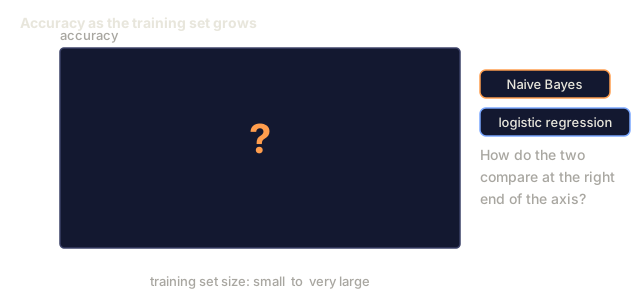
Naive Bayes vs Logistic Regression
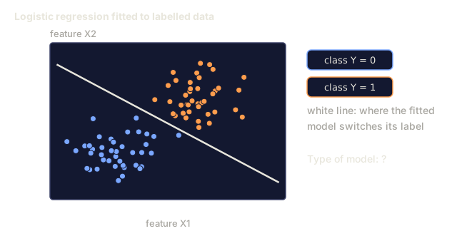
Both are linear classifiers for text. The difference is in what they model.
| Aspect | Naive Bayes | Logistic Regression |
|---|---|---|
| Type | Generative (models P(X|Y)) | Discriminative (models P(Y|X)) |
| Training | Count frequencies | Optimize loss function |
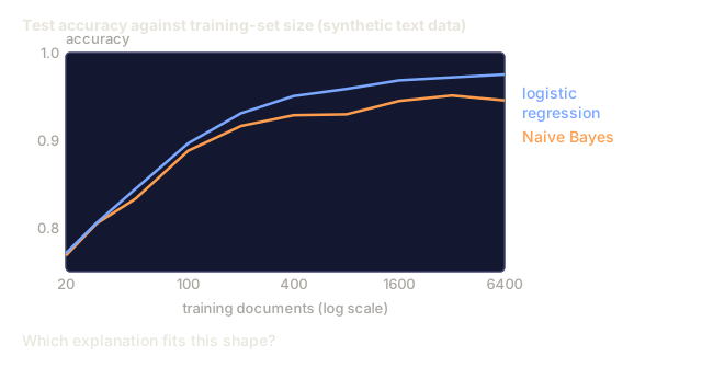
| Small data | Better (strong prior helps) | Worse (not enough to estimate weights) |
| Large data | Worse (wrong assumption hurts) | Better (flexible boundary) |
| Features | Assumes independence | Handles correlations |
| Speed | Single pass, very fast | Iterative optimization |
| Calibration | Poor probabilities | Better probabilities |
Rule of thumb: start with Naive Bayes. If you have enough data and NB plateaus, switch to logistic regression.
Classification Pipeline

This is the same log-space computation from above, laid out as a pipeline: sum the log prior and the log likelihoods for each class, then take the argmax.
log P(class | features) = log P(class) + sum_i log P(feature_i | class)


Build It
The code in code/naive_bayes.py implements both MultinomialNB and GaussianNB from scratch.
MultinomialNB
The from-scratch implementation:
-
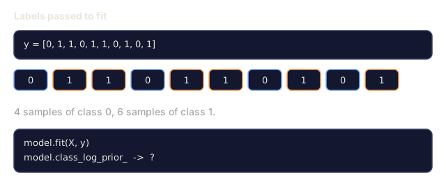
fit(X, y): For each class, count the frequency of each feature, add Laplace smoothing, compute log probabilities, and store the class priors (log of class frequencies).
-
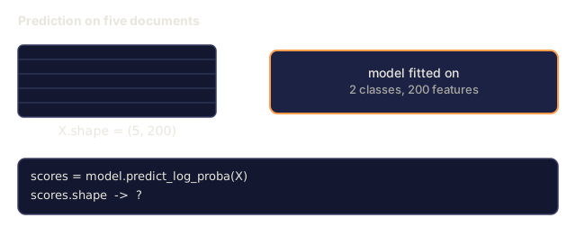
predict_log_proba(X): For each sample, compute log P(class) + sum of log P(feature_i | class) for all classes. This is a matrix multiplication: X @ log_probs.T + log_priors.
-
predict(X): Return the class with the highest log probability.
class MultinomialNB:
    def __init__(self, alpha=1.0):
        self.alpha = alpha

    def fit(self, X, y):
        classes = np.unique(y)
        n_classes = len(classes)
        n_features = X.shape[1]

        self.classes_ = classes
        self.class_log_prior_ = np.zeros(n_classes)
        self.feature_log_prob_ = np.zeros((n_classes, n_features))

        for i, c in enumerate(classes):
            X_c = X[y == c]
            self.class_log_prior_[i] = np.log(X_c.shape[0] / X.shape[0])
            counts = X_c.sum(axis=0) + self.alpha
            self.feature_log_prob_[i] = np.log(counts / counts.sum())

        return self
The key insight: once fitting is done, prediction is just matrix multiplication plus a bias. That's why Naive Bayes is so fast.
GaussianNB
For continuous features, we estimate mean and variance per class per feature:
class GaussianNB:
    def __init__(self):
        pass

    def fit(self, X, y):
        classes = np.unique(y)
        self.classes_ = classes
        self.means_ = np.zeros((len(classes), X.shape[1]))
        self.vars_ = np.zeros((len(classes), X.shape[1]))
        self.priors_ = np.zeros(len(classes))

        for i, c in enumerate(classes):
            X_c = X[y == c]
            self.means_[i] = X_c.mean(axis=0)
            self.vars_[i] = X_c.var(axis=0) + 1e-9
            self.priors_[i] = X_c.shape[0] / X.shape[0]

        return self
Prediction uses the Gaussian PDF per feature, multiplied across features (added in log space).
Demo: Text Classification
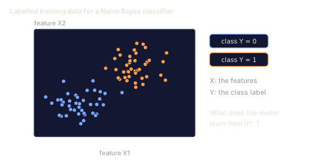
The code generates synthetic bag-of-words data simulating two classes (tech articles vs sports articles). Each class has a different word frequency distribution, and MultinomialNB classifies them using word counts.
The synthetic data works like this: we create 200 "words" (feature columns). Words 0-39 have high frequency in tech articles and low in sports. Words 80-119 have high frequency in sports and low in tech. Words 40-79 are medium frequency in both. This creates a realistic scenario where some words are strong class indicators and others are noise.
Demo: Continuous Features
The code generates Iris-like data (3 classes, 4 features, Gaussian clusters). GaussianNB classifies using per-class mean and variance. Each class has a different center (mean vector) and different spread (variance), mimicking real-world data where measurements differ systematically between categories.
The code also demonstrates:
- Smoothing comparison: training MultinomialNB with different alpha values to show the effect of smoothing strength on accuracy.
- Training size experiment: how NB accuracy improves as training data grows from 20 to 1600 samples. NB reaches decent accuracy even with very few samples, which is its main advantage.
- Confusion matrix: per-class precision, recall, and F1 score to show where NB makes mistakes.
Prediction Speed
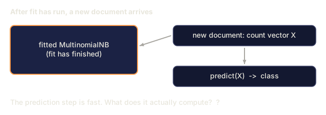
Naive Bayes prediction is a matrix multiplication. For n samples with d features and k classes:
- MultinomialNB: one matrix multiply (n x d) @ (d x k) = O(n * d * k)
- GaussianNB: n * k Gaussian PDF evaluations, each over d features = O(n * d * k)
Both are linear in every dimension. Compare that to KNN, which needs a distance computation against every training point, or an SVM with an RBF kernel, which needs a kernel evaluation against every support vector. NB is faster by orders of magnitude at prediction time.
Use It
With sklearn, both variants are one-liners:
from sklearn.naive_bayes import GaussianNB, MultinomialNB

gnb = GaussianNB()
gnb.fit(X_train, y_train)
print(f"GaussianNB accuracy: {gnb.score(X_test, y_test):.3f}")

mnb = MultinomialNB(alpha=1.0)
mnb.fit(X_train_counts, y_train)
print(f"MultinomialNB accuracy: {mnb.score(X_test_counts, y_test):.3f}")
For text classification with sklearn:
from sklearn.feature_extraction.text import CountVectorizer
from sklearn.naive_bayes import MultinomialNB
from sklearn.pipeline import Pipeline

text_clf = Pipeline([
    ("vectorizer", CountVectorizer()),
    ("classifier", MultinomialNB(alpha=1.0)),
])

text_clf.fit(train_texts, train_labels)
accuracy = text_clf.score(test_texts, test_labels)
The code in naive_bayes.py compares the from-scratch implementations against sklearn on the same data to verify correctness.
TF-IDF with Naive Bayes
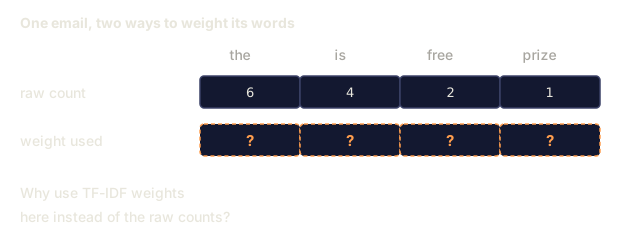
Raw word counts give every word equal weight per occurrence. But common words like "the" and "is" appear frequently in every class, so they carry no information. TF-IDF (Term Frequency - Inverse Document Frequency) downweights common words and upweights rare, discriminative words.
from sklearn.feature_extraction.text import TfidfVectorizer
from sklearn.naive_bayes import MultinomialNB
from sklearn.pipeline import Pipeline

text_clf = Pipeline([
    ("tfidf", TfidfVectorizer()),
    ("classifier", MultinomialNB(alpha=0.1)),
])
TF-IDF values are non-negative, so they work with MultinomialNB. The combination of TF-IDF and MultinomialNB is one of the strongest baselines for text classification. It frequently beats more complex models on datasets with fewer than 10,000 training samples.
BernoulliNB for Short Text
For short text (tweets, SMS, chat messages), BernoulliNB can outperform MultinomialNB. Short texts have low word counts, so the frequency information that MultinomialNB relies on is noisy. BernoulliNB only cares about presence or absence, which is more reliable with short text.
from sklearn.naive_bayes import BernoulliNB
from sklearn.feature_extraction.text import CountVectorizer

text_clf = Pipeline([
    ("vectorizer", CountVectorizer(binary=True)),
    ("classifier", BernoulliNB(alpha=1.0)),
])
The binary=True flag in CountVectorizer converts all counts to 0/1. Without it, BernoulliNB still works, but it's seeing counts it wasn't designed for.
Calibrating NB Probabilities
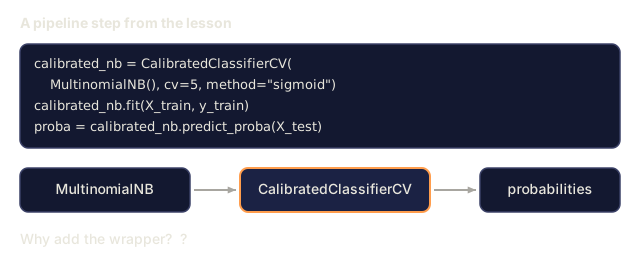
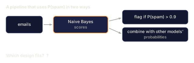
NB probabilities are poorly calibrated. When NB says P(spam) = 0.95, the true probability might be 0.7. If you need reliable probability estimates (for example, to set a threshold or to combine with other models), use sklearn's CalibratedClassifierCV:
from sklearn.calibration import CalibratedClassifierCV

calibrated_nb = CalibratedClassifierCV(MultinomialNB(), cv=5, method="sigmoid")
calibrated_nb.fit(X_train, y_train)
proba = calibrated_nb.predict_proba(X_test)
This fits a logistic regression on top of NB's raw scores using cross-validation. The resulting probabilities are much closer to the true class frequencies.
Common Gotchas
-
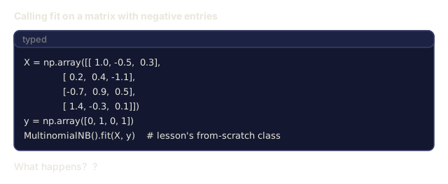
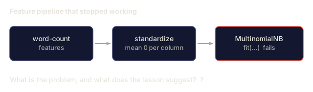
Negative feature values. MultinomialNB requires non-negative features. If you have negative values (like TF-IDF with certain settings or standardized features), use GaussianNB instead, or shift the features to be positive.
-
Zero variance features. GaussianNB divides by variance. If a feature has zero variance for a class (all values identical), the probability computation breaks. The code adds a small smoothing term (1e-9) to all variances to prevent this.
-
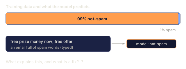
Class imbalance. If 99% of emails are not-spam, the prior P(not-spam) = 0.99 is so strong that it overwhelms the likelihood evidence. You can set class priors manually or use the class_prior parameter in sklearn.
-
Feature scaling. MultinomialNB doesn't need scaling (it works on counts). GaussianNB doesn't need scaling either (it estimates per-feature statistics). This is an advantage over logistic regression and SVM, both of which are sensitive to feature scales.
Ship It
This lesson produces:
outputs/skill-naive-bayes-chooser.md, a decision skill for picking the right NB variantcode/naive_bayes.py, MultinomialNB and GaussianNB from scratch, with a sklearn comparison
When Naive Bayes Fails
NB fails when the independence assumption causes incorrect rankings, not just incorrect probabilities. That happens when:
-
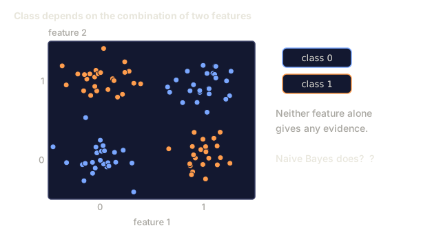
Strong feature interactions. If the class depends on the combination of two features but not either alone (XOR-like patterns), NB misses it entirely. Each feature alone provides no evidence, and NB can't combine them nonlinearly.
-
Highly correlated features with opposing evidence. If feature A says "spam" and feature B says "not-spam," but A and B are perfectly correlated (they always agree in reality), NB sees conflicting evidence where there is none.
-
Very large training sets. With enough data, discriminative models like logistic regression learn the true decision boundary and outperform NB. The independence assumption that helped with small data now holds the model back.
In practice, these failure modes are rare for text classification: text features are numerous, individually weak, and the independence assumption's errors tend to cancel out. For tabular data with a few strongly correlated features, reach for logistic regression or tree-based models first.
Exercises
-
Smoothing experiment. Train MultinomialNB on text data with alpha values of 0.01, 0.1, 1.0, 10.0, and 100.0. Plot accuracy vs alpha. Where does performance peak? Why does very high alpha hurt?
-
Feature independence test. Take a real text dataset. Pick two words that are obviously correlated ("machine" and "learning"). Compute P(word1 | class) * P(word2 | class) and compare to P(word1 AND word2 | class). How wrong is the independence assumption? Does it affect classification accuracy?
-
Bernoulli implementation. Extend the code with a BernoulliNB class. Convert bag-of-words to binary (present/absent) and compare accuracy against MultinomialNB on text data. When does Bernoulli win?
-
NB vs Logistic Regression. Train both on text data. Start with 100 training samples and increase to 10,000. Plot accuracy vs training set size for both. At what point does Logistic Regression overtake Naive Bayes?
-
Spam filter. Build a complete spam classifier: tokenize raw email text, build vocabulary, create bag-of-words features, train MultinomialNB, evaluate with precision and recall (not just accuracy — why?).
Key Terms
| Term | What people say | What it actually means |
|---|---|---|
| Naive Bayes | "Simple probabilistic classifier" | A classifier that applies Bayes' theorem with the assumption that features are conditionally independent given the class |
| Conditional independence | "Features don't affect each other" | P(A, B | C) = P(A | C) * P(B | C): knowing B tells you nothing new about A once you know C |
| Laplace smoothing | "Add-one smoothing" | Adding a small count to every feature to prevent zero probabilities from dominating the prediction |
| Prior | "What you believed before seeing data" | P(class): the probability of each class before observing any features |
| Likelihood | "How well the data fits" | P(features | class): the probability of observing these features if the class is known |
| Posterior | "What you believe after seeing data" | P(class | features): the updated probability of the class after observing the features |
| Generative model | "Models how data is generated" | A model that learns P(X | Y) and P(Y), then uses Bayes' theorem to get P(Y | X) |
| Discriminative model | "Models the decision boundary" | A model that directly learns P(Y | X) without modeling how X is generated |
| Log probability | "Avoid underflow" | Working with log P instead of P to prevent the product of many small numbers from becoming zero in floating point |
Further Reading
- scikit-learn Naive Bayes docs — all three variants with mathematical details
- McCallum and Nigam, A Comparison of Event Models for Naive Bayes Text Classification (1998) — the classic comparison of Multinomial vs Bernoulli for text
- Rennie et al., Tackling the Poor Assumptions of Naive Bayes Text Classifiers (2003) — improvements to NB for text
- Ng and Jordan, On Discriminative vs. Generative Classifiers (2001) — proves NB converges faster than LR with less data
Code
- naive_bayes.py (python, 345 lines)