Probability and Distributions
Probability is the only language a model has for saying 'I'm not sure.'
Learning Objectives
- Implement PMFs and PDFs from scratch for Bernoulli, categorical, Poisson, uniform, and normal distributions
- Compute expected value, variance, and use the Central Limit Theorem to explain why Gaussians dominate
- Build softmax and log-softmax functions with the numerical stability trick (subtract max logit)
- Calculate cross-entropy loss from logits and connect it to negative log-likelihood
The Problem
A classifier outputs [0.03, 0.91, 0.06]. A language model picks its next token out of 50,000 candidates. A diffusion model paints an image by repeatedly sampling from a distribution it learned during training. Different tasks, same underlying move: probability in action.
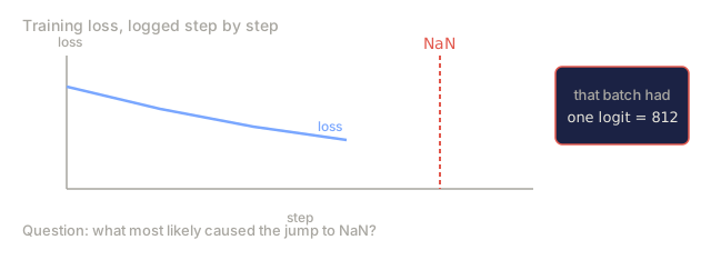
That move never stops. A model's prediction is a probability distribution, its loss function is a measure of distance between that distribution and the true one, and every training step is just nudging one distribution to look more like the other. Skip probability and you can't read an ML paper, you can't debug a model that's gone wrong, and you definitely can't explain why your training loss just turned into NaN.
The Concept
Events, Sample Spaces, and Probability
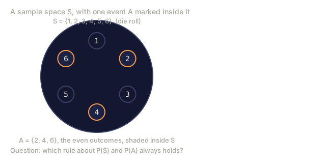
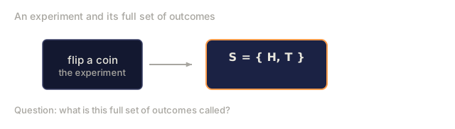
The sample space S is the set of every possible outcome. An event is any subset of that space, and probability is the function that maps each event to a number between 0 and 1.
Coin flip:
  S = {H, T}
  P(H) = 0.5,  P(T) = 0.5

Single die roll:
  S = {1, 2, 3, 4, 5, 6}
  P(even) = P({2, 4, 6}) = 3/6 = 0.5
Three axioms define the entire subject:
- P(A) >= 0 for any event A
- P(S) = 1 (something always happens)
- P(A or B) = P(A) + P(B) when A and B cannot both occur
Bayes' theorem, expected value, every distribution in this lesson: all of it follows from these three rules.
Conditional Probability and Independence
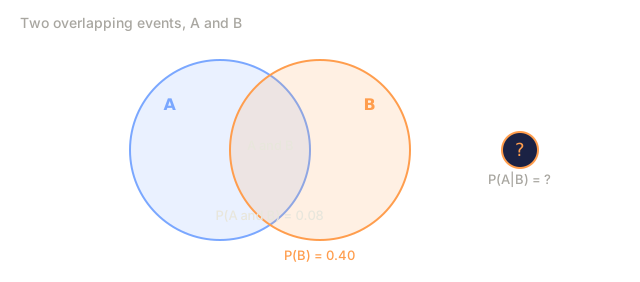
P(A|B) is the probability of A, given that B already happened.
P(A|B) = P(A and B) / P(B)

Example: deck of cards
  P(King | Face card) = P(King and Face card) / P(Face card)
                      = (4/52) / (12/52)
                      = 4/12 = 1/3
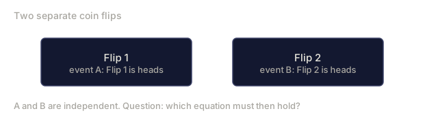
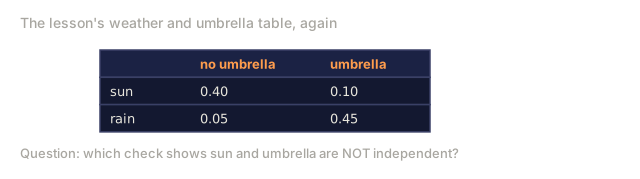
Two events are independent exactly when knowing one tells you nothing about the other:
Independent:   P(A|B) = P(A)
Equivalent to: P(A and B) = P(A) * P(B)
Coin flips are independent of each other. Drawing cards without replacement is not.
Probability Mass Functions vs Probability Density Functions
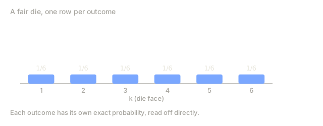
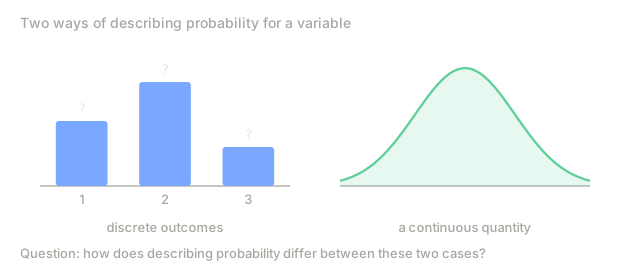
A discrete random variable has a probability mass function (PMF): every outcome carries a specific probability you can read off directly.
PMF: P(X = k)

Fair die:
  P(X = 1) = 1/6
  P(X = 2) = 1/6
  ...
  P(X = 6) = 1/6

  Sum of all probabilities = 1
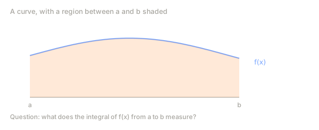
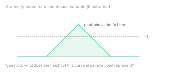
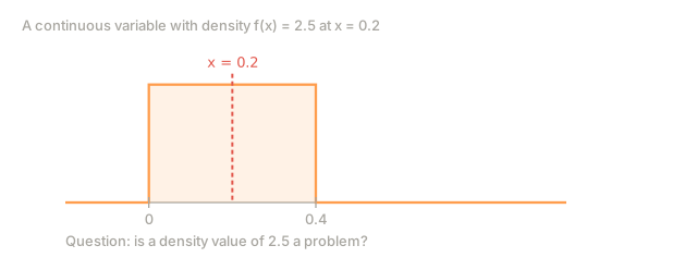
A continuous random variable has a probability density function (PDF) instead. The density at any single point isn't itself a probability; you only get a probability by integrating that density over an interval.
PDF: f(x)

P(a <= X <= b) = integral of f(x) from a to b

f(x) can be greater than 1 (density, not probability)
integral from -inf to +inf of f(x) dx = 1
The distinction matters in ML. Classification is a discrete choice, so its outputs are PMFs. Take a VAE (variational autoencoder, a generative model that learns a compressed representation of data): its latent space is continuous, so it works with PDFs.
Common Distributions
Bernoulli: one trial, two outcomes. This is the distribution binary classification runs on.
P(X = 1) = p
P(X = 0) = 1 - p
Mean = p,  Variance = p(1-p)
Categorical: one trial, k possible outcomes, exactly what softmax hands you for multi-class classification.
P(X = i) = p_i,  where sum of p_i = 1
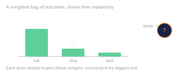
Example: P(cat) = 0.7,  P(dog) = 0.2,  P(bird) = 0.1
Uniform: every outcome equally likely. The default for random initialization.
Discrete: P(X = k) = 1/n for k in {1, ..., n}
Continuous: f(x) = 1/(b-a) for x in [a, b]
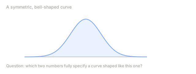
Normal (Gaussian): the bell curve, set by two numbers, mean (mu) and variance (sigma^2).
f(x) = (1 / sqrt(2*pi*sigma^2)) * exp(-(x - mu)^2 / (2*sigma^2))

Standard normal: mu = 0, sigma = 1
  68% of data within 1 sigma
  95% within 2 sigma
  99.7% within 3 sigma
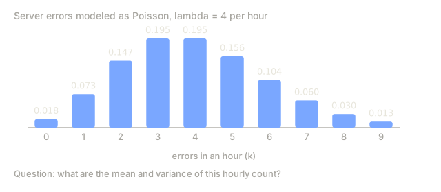
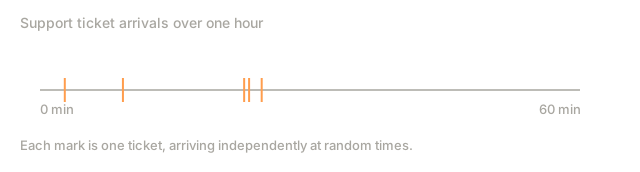
Poisson: counts of rare events over a fixed interval. This is the distribution behind event rates.
P(X = k) = (lambda^k * e^(-lambda)) / k!
Mean = lambda,  Variance = lambda
Expected Value and Variance
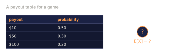
Expected value is the probability-weighted average outcome.
Discrete:   E[X] = sum of x_i * P(X = x_i)
Continuous: E[X] = integral of x * f(x) dx
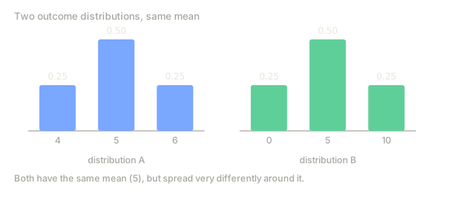
Variance measures how spread out the outcomes are around that mean.
Var(X) = E[(X - E[X])^2] = E[X^2] - (E[X])^2
Standard deviation = sqrt(Var(X))
In ML, the loss function you're minimizing is an expected value: the average loss over the data distribution. Variance shows up as a stability signal instead. When your gradients have high variance, training gets noisy.
Joint and Marginal Distributions
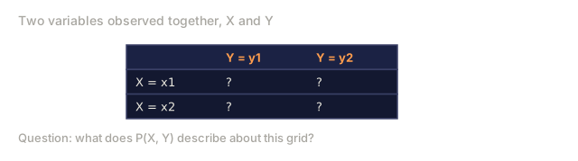
A joint distribution, P(X, Y), describes two random variables at once.
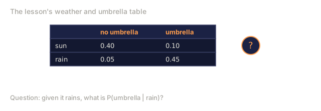
Joint PMF example (X = weather, Y = umbrella):
| Y=0 (no umbrella) | Y=1 (umbrella) | Marginal P(X) | |
|---|---|---|---|
| X=0 (sun) | 0.40 | 0.10 | P(X=0) = 0.50 |
| X=1 (rain) | 0.05 | 0.45 | P(X=1) = 0.50 |
| Marginal P(Y) | P(Y=0) = 0.45 | P(Y=1) = 0.55 | 1.00 |
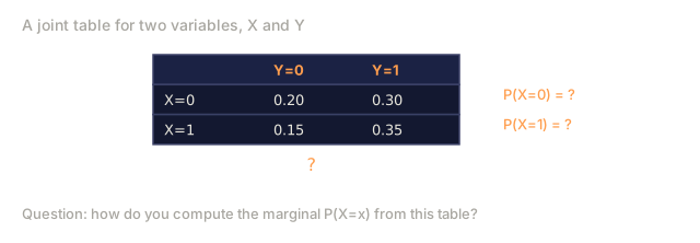
The marginal distribution sums out the other variable:
P(X = x) = sum over all y of P(X = x, Y = y)
Those row and column totals in the table above are exactly the marginals.
Why the Normal Distribution Shows Up Everywhere
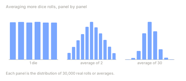
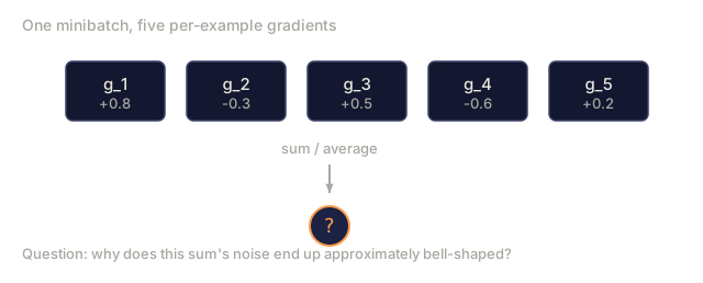
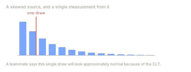
The Central Limit Theorem: the sum, or average, of many independent random variables converges to a normal distribution, no matter what distribution you started with.
Roll 1 die:  uniform distribution (flat)
Average of 2 dice:  triangular (peaked)
Average of 30 dice: nearly perfect bell curve

This works for ANY starting distribution.
That's why:
- Measurement errors are approximately normal (many small independent sources)
- Weight initializations in neural networks use normal distributions
- Gradient noise in SGD (stochastic gradient descent) is approximately normal (sum of many sample gradients)
- The normal distribution is the maximum entropy distribution for a given mean and variance
Log Probabilities
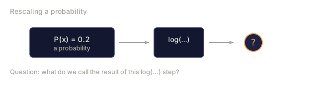
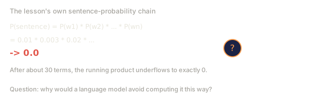
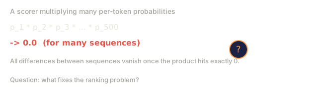
A log probability is log(P(x)): the same probability, just expressed on a log scale. Here's why that's worth doing. Raw probabilities break down numerically — multiply enough small ones together and the product underflows to zero:
P(sentence) = P(word1) * P(word2) * ... * P(word_n)
            = 0.01 * 0.003 * 0.02 * ...
            -> 0.0 (underflow after ~30 terms)
Taking the log turns that multiplication into addition, and addition doesn't underflow:
log P(sentence) = log P(word1) + log P(word2) + ... + log P(word_n)
                = -4.6 + -5.8 + -3.9 + ...
                -> finite number (no underflow)
Rules:
- log(a * b) = log(a) + log(b)
- log probabilities are always <= 0 (since 0 < P <= 1)
- more negative means less likely
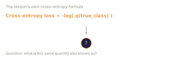
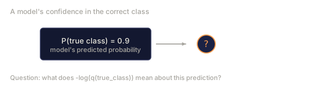
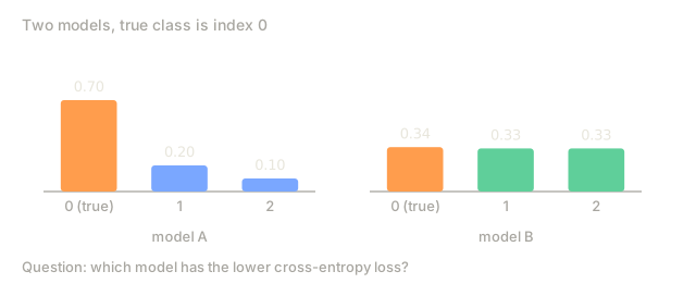
- cross-entropy loss is the negative log probability of the correct class, also called the negative log-likelihood
Softmax as a Probability Distribution
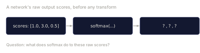
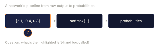
A neural network's raw output is a set of scores called logits. Softmax is the function that turns those logits into a valid probability distribution:
softmax(z_i) = exp(z_i) / sum(exp(z_j) for all j)

Properties:
  - All outputs are in (0, 1)
  - All outputs sum to 1
  - Preserves relative ordering of inputs
  - exp() amplifies differences between logits
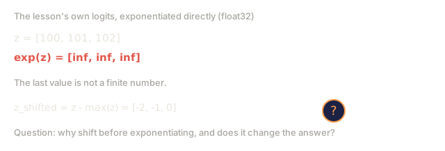
The softmax trick: subtract the max logit before you exponentiate, so nothing overflows.
z = [100, 101, 102]
exp(102) = overflow

z_shifted = z - max(z) = [-2, -1, 0]
exp(0) = 1  (safe)

Same result, no overflow.
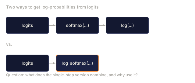
Log-softmax fuses softmax and log into one numerically stable operation. PyTorch runs this internally for cross-entropy loss.
Sampling
Sampling is drawing random values from a distribution. In ML, it shows up constantly:
- Dropout randomly samples which neurons to zero out
- Data augmentation samples random transformations
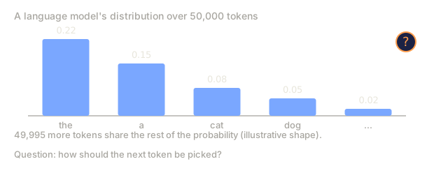
- Language models sample the next token from the predicted distribution
- Diffusion models sample noise and progressively denoise
Sampling from an arbitrary distribution isn't always trivial. It takes techniques like inverse transform sampling, rejection sampling, or the reparameterization trick VAEs rely on.

Build It
Step 1: Probability basics
import math
import random

def factorial(n):
    result = 1
    for i in range(2, n + 1):
        result *= i
    return result

def combinations(n, k):
    return factorial(n) // (factorial(k) * factorial(n - k))

def conditional_probability(p_a_and_b, p_b):
    return p_a_and_b / p_b

p_king_given_face = conditional_probability(4/52, 12/52)
print(f"P(King | Face card) = {p_king_given_face:.4f}")
Step 2: PMF and PDF from scratch
def bernoulli_pmf(k, p):
    return p if k == 1 else (1 - p)

def categorical_pmf(k, probs):
    return probs[k]

def poisson_pmf(k, lam):
    return (lam ** k) * math.exp(-lam) / factorial(k)

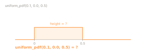
def uniform_pdf(x, a, b):
    if a <= x <= b:
        return 1.0 / (b - a)
    return 0.0

def normal_pdf(x, mu, sigma):
    coeff = 1.0 / (sigma * math.sqrt(2 * math.pi))
    exponent = -0.5 * ((x - mu) / sigma) ** 2
    return coeff * math.exp(exponent)
Step 3: Expected value and variance
def expected_value(values, probabilities):
    return sum(v * p for v, p in zip(values, probabilities))

def variance(values, probabilities):
    mu = expected_value(values, probabilities)
    return sum(p * (v - mu) ** 2 for v, p in zip(values, probabilities))

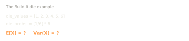
die_values = [1, 2, 3, 4, 5, 6]
die_probs = [1/6] * 6
mu = expected_value(die_values, die_probs)
var = variance(die_values, die_probs)
print(f"Die: E[X] = {mu:.4f}, Var(X) = {var:.4f}, SD = {var**0.5:.4f}")
Step 4: Sampling from distributions
def sample_bernoulli(p, n=1):
    return [1 if random.random() < p else 0 for _ in range(n)]

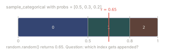
def sample_categorical(probs, n=1):
    cumulative = []
    total = 0
    for p in probs:
        total += p
        cumulative.append(total)
    samples = []
    for _ in range(n):
        r = random.random()
        for i, c in enumerate(cumulative):
            if r <= c:
                samples.append(i)
                break
    return samples

def sample_normal_box_muller(mu, sigma, n=1):
    samples = []
    for _ in range(n):
        u1 = random.random()
        u2 = random.random()
        z = math.sqrt(-2 * math.log(u1)) * math.cos(2 * math.pi * u2)
        samples.append(mu + sigma * z)
    return samples
Step 5: Softmax and log probabilities
def softmax(logits):
    max_logit = max(logits)
    shifted = [z - max_logit for z in logits]
    exps = [math.exp(z) for z in shifted]
    total = sum(exps)
    return [e / total for e in exps]

def log_softmax(logits):
    max_logit = max(logits)
    shifted = [z - max_logit for z in logits]
    log_sum_exp = max_logit + math.log(sum(math.exp(z) for z in shifted))
    return [z - log_sum_exp for z in logits]

def cross_entropy_loss(logits, target_index):
    log_probs = log_softmax(logits)
    return -log_probs[target_index]
Step 6: Central Limit Theorem demonstration
def demonstrate_clt(dist_fn, n_samples, n_averages):
    averages = []
    for _ in range(n_averages):
        samples = [dist_fn() for _ in range(n_samples)]
        averages.append(sum(samples) / len(samples))
    return averages
Step 7: Visualization
import matplotlib.pyplot as plt

xs = [mu + sigma * (i - 500) / 100 for i in range(1001)]
ys = [normal_pdf(x, mu, sigma) for x, mu, sigma in ...]
plt.plot(xs, ys)
The full implementation, with every visualization, lives in code/probability.py.




Use It
With NumPy and SciPy, everything above collapses to one-liners:
import numpy as np
from scipy import stats

normal = stats.norm(loc=0, scale=1)
samples = normal.rvs(size=10000)
print(f"Mean: {np.mean(samples):.4f}, Std: {np.std(samples):.4f}")
print(f"P(X < 1.96) = {normal.cdf(1.96):.4f}")

logits = np.array([2.0, 1.0, 0.1])
from scipy.special import softmax, log_softmax
probs = softmax(logits)
log_probs = log_softmax(logits)
print(f"Softmax: {probs}")
print(f"Log-softmax: {log_probs}")
You built all of this by hand first. Now you know exactly what the library call is doing underneath.
The first time I watched a model's loss jump to nan mid-training, I assumed I'd broken something in the architecture. I hadn't. Somewhere in that batch, softmax had exponentiated a large logit into infinity, or a log() call had been handed a probability of exactly zero, and the whole computation graph poisoned itself from that point on. Every fix for this traces straight back to this lesson: shift the logits down before exponentiating, do your arithmetic in log space instead of raw probabilities, never let anything touch log(0) unguarded. None of it is exotic math. It's the boring numerical hygiene that keeps a training run from quietly going wrong for three hours before you notice the loss curve went flat. Learn the shift-and-log trick once, here, and you'll spot this bug on sight for the rest of your career.
Exercises
-
Implement inverse transform sampling for the exponential distribution. Verify by sampling 10,000 values and comparing the histogram to the true PDF.
-
Build a joint distribution table for two loaded dice. Compute the marginal distributions and check whether the dice are independent.
-
Compute the cross-entropy loss for a 5-class classifier that outputs logits
[2.0, 0.5, -1.0, 3.0, 0.1]when the correct class is index 3. Then verify your answer with PyTorch'snn.CrossEntropyLoss. -
Write a function that takes a list of log probabilities and returns the most likely sequence, the total log probability, and the equivalent raw probability. Test it with a sentence of 50 words where each word has probability 0.01.
Key Terms
| Term | What people say | What it actually means |
|---|---|---|
| Sample space | "All the possibilities" | The set S of every possible outcome of an experiment |
| PMF | "The probability function" | A function that gives the exact probability of each discrete outcome, summing to 1 |
| "The probability curve" | A density function for continuous variables. Integrate it over an interval to get probability | |
| Conditional probability | "Probability given something" | P(A|B) = P(A and B) / P(B). The foundation of Bayesian thinking and Bayes' theorem |
| Independence | "They don't affect each other" | P(A and B) = P(A) * P(B). Knowing one event tells you nothing about the other |
| Expected value | "The average" | The probability-weighted sum of all outcomes. The loss function is an expected value |
| Variance | "How spread out" | The expected squared deviation from the mean. High variance = noisy, unstable estimates |
| Normal distribution | "The bell curve" | f(x) = (1/sqrt(2pisigma^2)) * exp(-(x-mu)^2/(2*sigma^2)). Appears everywhere due to the CLT |
| Central Limit Theorem | "Averages become normal" | The mean of many independent samples converges to a normal distribution regardless of the source |
| Joint distribution | "Two variables together" | P(X, Y) describes the probability of every combination of X and Y outcomes |
| Marginal distribution | "Sum out the other variable" | P(X) = sum_y P(X, Y). Recovers one variable's distribution from the joint |
| Log probability | "Log of the probability" | log P(x). Turns products into sums, preventing numerical underflow in long sequences |
| Softmax | "Turn scores into probabilities" | softmax(z_i) = exp(z_i) / sum(exp(z_j)). Maps real-valued logits to a valid probability distribution |
| Cross-entropy | "The loss function" | -sum(p_true * log(p_predicted)), the negative log-likelihood of the correct class. Measures how different two distributions are. Lower is better |
| Logits | "Raw model outputs" | Unnormalized scores before softmax. Named after the logistic function |
| Sampling | "Drawing random values" | Generating values according to a probability distribution. How models generate output |
Further Reading
- 3Blue1Brown: But what is the Central Limit Theorem? — visual proof of why averages become normal
- Stanford CS229 Probability Review — concise reference covering everything here and more
- The Log-Sum-Exp Trick — why numerical stability matters and how to achieve it
Code
- main.jl (text, 285 lines)
- probability.py (python, 327 lines)