Sampling Methods
Every generative model (LLM, diffusion, GAN) is just a sampling algorithm wearing a costume.
Learning Objectives
- Implement inverse CDF, rejection, and importance sampling from scratch using only uniform random numbers
- Build temperature, top-k, and top-p (nucleus) sampling for language model token generation
- Explain the reparameterization trick and why it enables backpropagation through sampling in VAEs
- Run Metropolis-Hastings MCMC to sample from an unnormalized target distribution
The Problem
A language model finishes processing your prompt and produces a vector of 50,000 logits, one for every token in its vocabulary. Now it has to pick one. How?
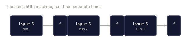
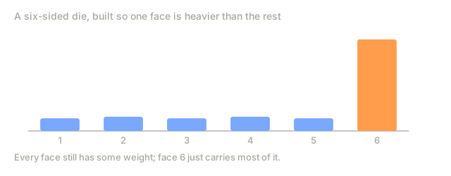
Always take the highest-probability token and every response comes out identical: deterministic, safe, boring. Pick uniformly at random instead and you get gibberish. The useful answer sits somewhere between those two extremes, and sampling is what decides exactly where.
Sampling isn't just a text-generation trick. Reinforcement learning estimates policy gradients by sampling trajectories. VAEs learn latent representations by sampling from a learned distribution and backpropagating through the randomness. Diffusion models generate images by sampling noise and denoising it step by step. Monte Carlo methods estimate integrals that have no closed form. MCMC explores posterior distributions too high-dimensional to enumerate directly.
Every generative AI system, underneath, is a sampling system. The sampling strategy is what decides the quality, diversity, and controllability of what comes out. This lesson builds every major sampling method from scratch, starting from uniform random numbers and ending at the techniques running inside modern LLMs and generative models.
The Concept
Why Sampling Matters
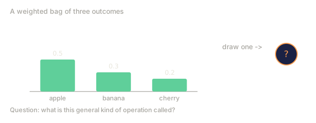
Sampling is the act of generating values according to a probability distribution instead of just picking the one you think is right. It shows up in four fundamental roles across AI and machine learning.
Generation. Language models, diffusion models, and GANs all produce output by sampling. A GAN's generator starts from a latent vector sampled from a simple prior, usually a standard normal, and maps it into an image, so the sample drawn fully determines what comes out. The sampling algorithm directly controls creativity, coherence, and diversity, and temperature, top-k, and nucleus sampling are the knobs engineers turn every day.
Training. Stochastic gradient descent samples mini-batches. Dropout samples which neurons to deactivate. Data augmentation samples random transformations. Importance sampling reweights samples to cut gradient variance in reinforcement learning (PPO, TRPO, both trust-region policy-gradient methods).
Estimation. Plenty of quantities in ML have no closed-form solution: the expected loss over a data distribution, the partition function of an energy-based model, the evidence in Bayesian inference. Monte Carlo estimation approximates all of these by averaging over samples.
Exploration. MCMC explores posterior distributions in Bayesian inference. Evolutionary strategies sample parameter perturbations. Thompson sampling balances exploration against exploitation in bandits.
The core challenge is that you can only sample directly from simple distributions like uniform and normal. For everything else, you need a method that converts those simple samples into samples from whatever distribution you actually care about.
Uniform Random Sampling
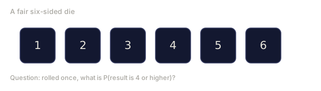
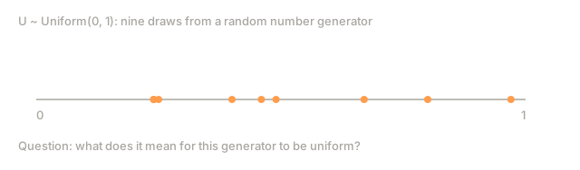
Every sampling method starts here. A uniform random number generator produces values in [0, 1), where every sub-interval of equal length has equal probability.
U ~ Uniform(0, 1)

P(a <= U <= b) = b - a    for 0 <= a <= b <= 1

Properties:
  E[U] = 0.5
  Var(U) = 1/12
To sample uniformly from a discrete set of n items, generate U and return floor(n * U). To sample from a continuous range [a, b], compute a + (b - a) * U.
Here's the key insight: a single uniform random number carries exactly enough randomness to produce one sample from any distribution you like. The trick is finding the right transformation.
Inverse CDF Method (Inverse Transform Sampling)
The cumulative distribution function (CDF) maps values to probabilities:
F(x) = P(X <= x)

Properties:
  F is non-decreasing
  F(-inf) = 0
  F(+inf) = 1
  F maps the real line to [0, 1]
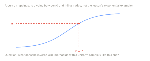
The inverse CDF maps probabilities back to values. If U ~ Uniform(0, 1), then X = F_inverse(U) follows the target distribution.
Algorithm:
  1. Generate u ~ Uniform(0, 1)
  2. Return F_inverse(u)

Why it works:
  P(X <= x) = P(F_inverse(U) <= x) = P(U <= F(x)) = F(x)
Exponential distribution example:
PDF: f(x) = lambda * exp(-lambda * x),   x >= 0
CDF: F(x) = 1 - exp(-lambda * x)

Solve F(x) = u for x:
  u = 1 - exp(-lambda * x)
  exp(-lambda * x) = 1 - u
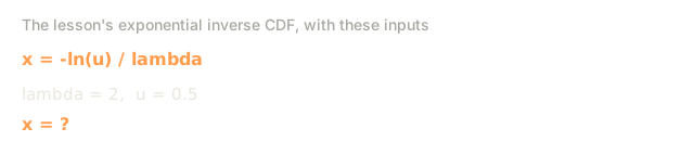
  x = -ln(1 - u) / lambda

Since (1 - U) and U have the same distribution:
  x = -ln(u) / lambda
This works perfectly when you can write F_inverse in closed form. The normal distribution has no closed-form inverse CDF, so it needs other methods instead (Box-Muller, or a numerical approximation).
Discrete version: For discrete distributions, build the CDF as a cumulative sum, generate U, and find the first index where the cumulative sum exceeds U. This is how sample_categorical works in Lesson 06.
Rejection Sampling
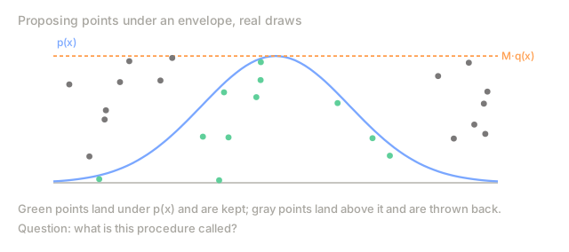
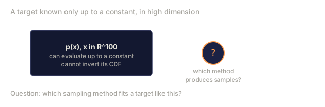
Rejection sampling works when you cannot invert the CDF, but you can still evaluate the target PDF up to a constant.
Target distribution: p(x)  (can evaluate, possibly unnormalized)
Proposal distribution: q(x)  (can sample from)
Bound: M such that p(x) <= M * q(x) for all x

Algorithm:
  1. Sample x ~ q(x)
  2. Sample u ~ Uniform(0, 1)
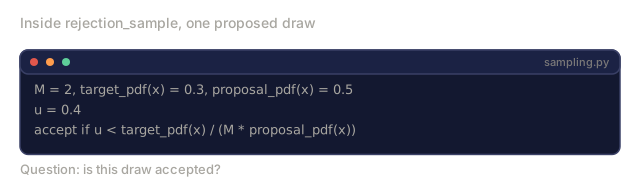
  3. If u < p(x) / (M * q(x)), accept x
  4. Otherwise, reject and go to step 1

Acceptance rate = 1/M
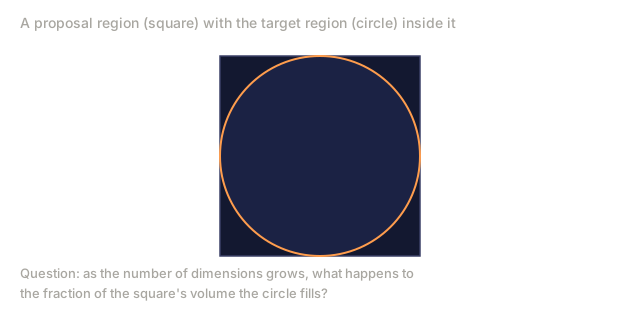
The tighter the bound M, the higher the acceptance rate. Rejection sampling works well in low dimensions (1 to 3). In high dimensions, the acceptance rate drops exponentially because almost all of the proposal volume gets rejected. That's the curse of dimensionality, showing up here for rejection sampling specifically.
Example: sampling from a truncated normal. Use a uniform proposal over the truncated range. The envelope M is the maximum of the normal PDF in that range.
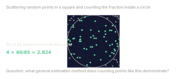
Example: sampling from a semicircle. Propose uniformly in the bounding rectangle. Accept if the point falls inside the semicircle. This is how Monte Carlo computes pi: the acceptance rate equals the area ratio pi/4.
Importance Sampling
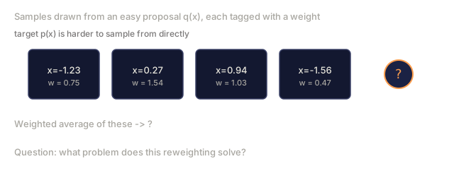
Importance sampling estimates an expectation under a target distribution p(x) using samples drawn from a different, easier-to-sample distribution q(x). You never need to draw a single sample from p(x) itself.
Goal: estimate E_p[f(x)] = integral of f(x) * p(x) dx

Rewrite:
  E_p[f(x)] = integral of f(x) * (p(x)/q(x)) * q(x) dx
            = E_q[f(x) * w(x)]

where w(x) = p(x) / q(x)  are the importance weights.

Estimator:
  E_p[f(x)] ~ (1/N) * sum(f(x_i) * w(x_i))    where x_i ~ q(x)
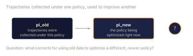
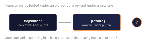
This is exactly what reinforcement learning needs. In PPO (Proximal Policy Optimization), you collect trajectories under an old policy pi_old but want to optimize a new policy pi_new. The importance weight is pi_new(a|s) / pi_old(a|s), and PPO clips these weights so the new policy can't drift too far from the old one.
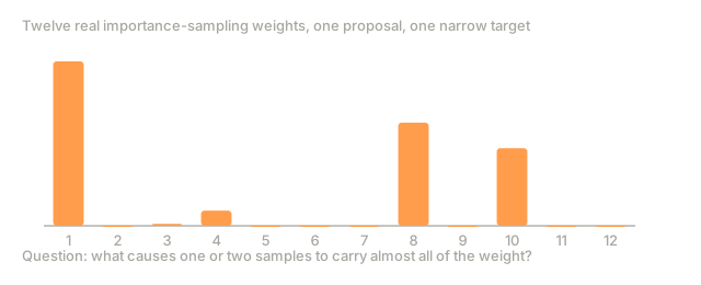
The estimator's variance depends on how close q is to p. When q is very different from p, a handful of samples pick up enormous weights and dominate the whole estimate. Self-normalized importance sampling divides by the sum of the weights to soften that problem:
E_p[f(x)] ~ sum(w_i * f(x_i)) / sum(w_i)
Monte Carlo Estimation
Monte Carlo estimation approximates integrals by averaging random samples, and the law of large numbers guarantees it converges.
Goal: estimate I = integral of g(x) dx over domain D

Method:
  1. Sample x_1, ..., x_N uniformly from D
  2. I ~ (Volume of D / N) * sum(g(x_i))

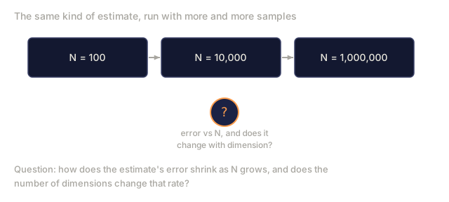
Error: O(1 / sqrt(N))   regardless of dimension
That error rate doesn't care about dimension at all, which is exactly why Monte Carlo dominates in high-dimensional settings where grid-based integration falls apart.
Estimating pi:
Sample (x, y) uniformly from [-1, 1] x [-1, 1]
Count how many fall inside the unit circle: x^2 + y^2 <= 1
pi ~ 4 * (count inside) / (total count)
Estimating expectations:
E[f(X)] ~ (1/N) * sum(f(x_i))    where x_i ~ p(x)

The sample mean converges to the true expectation.
Variance of the estimator = Var(f(X)) / N
Markov Chain Monte Carlo (MCMC): Metropolis-Hastings
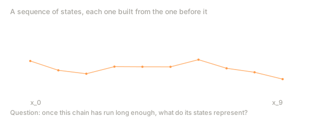
MCMC constructs a Markov chain whose stationary distribution is the target distribution p(x). After enough steps, samples from the chain are (approximately) samples from p(x).
Target: p(x)  (known up to a normalizing constant)
Proposal: q(x'|x)  (how to propose the next state given the current state)

Metropolis-Hastings algorithm:
  1. Start at some x_0
  2. For t = 1, 2, ..., T:
     a. Propose x' ~ q(x'|x_t)
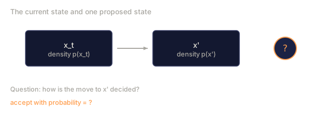
     b. Compute acceptance ratio:
        alpha = [p(x') * q(x_t|x')] / [p(x_t) * q(x'|x_t)]
     c. Accept with probability min(1, alpha):
        - If u < alpha (u ~ Uniform(0,1)): x_{t+1} = x'
        - Otherwise: x_{t+1} = x_t
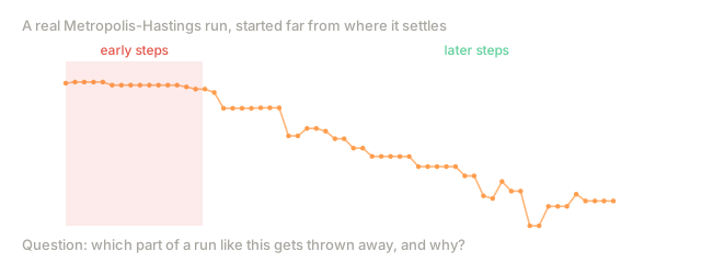
  3. Discard first B samples (burn-in)
  4. Return remaining samples
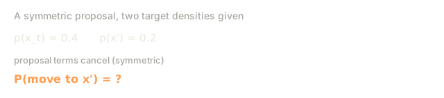
For symmetric proposals, where q(x'|x) equals q(x|x'), the ratio collapses to p(x')/p(x). That's the original Metropolis algorithm.
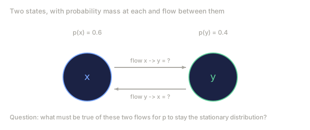
Why it works. The acceptance rule ensures detailed balance: the probability of being at x and moving to x' equals the probability of being at x' and moving to x. Detailed balance implies that p(x) is the stationary distribution of the chain.
Practical considerations:
- Burn-in: discard early samples before the chain reaches equilibrium
- Thinning: keep every k-th sample to reduce autocorrelation
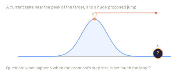
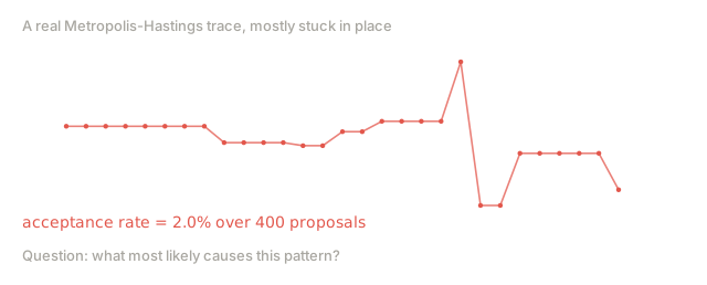
- Proposal scale: too small and the chain moves slowly (high acceptance, slow exploration); too large and most proposals are rejected (low acceptance, stuck in place)
- The optimal acceptance rate for a Gaussian proposal in high dimensions is approximately 0.234
Gibbs Sampling
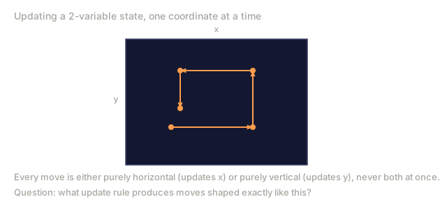
Gibbs sampling is a special case of MCMC for multivariate distributions. Instead of proposing a move in all dimensions at once, it updates one variable at a time from its conditional distribution.
Target: p(x_1, x_2, ..., x_d)

Algorithm:
  For each iteration t:
    Sample x_1^{t+1} ~ p(x_1 | x_2^t, x_3^t, ..., x_d^t)
    Sample x_2^{t+1} ~ p(x_2 | x_1^{t+1}, x_3^t, ..., x_d^t)
    ...
    Sample x_d^{t+1} ~ p(x_d | x_1^{t+1}, x_2^{t+1}, ..., x_{d-1}^{t+1})
Gibbs sampling needs you to be able to sample from each conditional distribution p(x_i | x_{-i}), which is straightforward for plenty of models:
- Bayesian networks: conditionals follow from the graph structure
- Gaussian mixtures: conditionals are Gaussian
- Ising models: each spin's conditional depends only on its neighbors
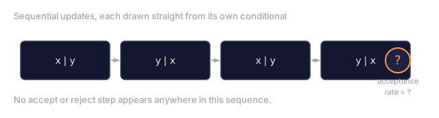
Its acceptance rate is always 1 (every proposal gets accepted) because sampling from the exact conditional automatically satisfies detailed balance.
Limitation. When variables are highly correlated, Gibbs sampling mixes slowly because updating one variable at a time cannot make large diagonal moves through the distribution.
Temperature Sampling (Used in LLMs)
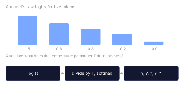
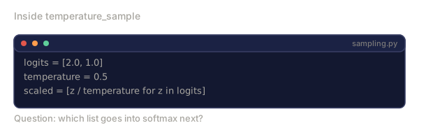
Language models output logits z_1, ..., z_V for each token in the vocabulary. Softmax converts these to probabilities. Temperature rescales the logits before softmax:
p_i = exp(z_i / T) / sum(exp(z_j / T))

T = 1.0: standard softmax (original distribution)
T -> 0:  argmax (deterministic, always picks highest logit)
T -> inf: uniform (all tokens equally likely)
T < 1.0: sharpens the distribution (more confident, less diverse)
T > 1.0: flattens the distribution (less confident, more diverse)
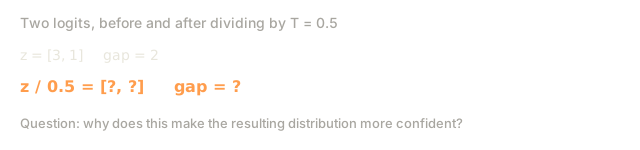
Why it works. Dividing logits by T < 1 amplifies differences between logits. If z_1 = 2 and z_2 = 1, dividing by T = 0.5 gives z_1/T = 4 and z_2/T = 2, making the gap larger. After softmax, the highest-logit token gets a much larger share.
In practice:
- T = 0.0: greedy decoding, best for factual Q&A
- T = 0.3-0.7: slightly creative, good for code generation
- T = 0.7-1.0: balanced, good for general conversation
- T = 1.0-1.5: creative writing, brainstorming
- T > 1.5: increasingly random, rarely useful
Temperature does not change which tokens are possible. It changes the probability mass allocated to each token.
Top-k Sampling
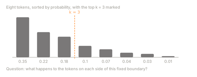
Top-k sampling restricts the candidate set to the k tokens with the highest probabilities, then renormalizes and samples from that restricted set.
Algorithm:
  1. Compute softmax probabilities for all V tokens
  2. Sort tokens by probability (descending)
  3. Keep only the top k tokens
  4. Renormalize: p_i' = p_i / sum(p_j for j in top-k)
  5. Sample from the renormalized distribution

k = 1:  greedy decoding
k = V:  no filtering (standard sampling)
k = 40: typical setting, removes long tail of unlikely tokens
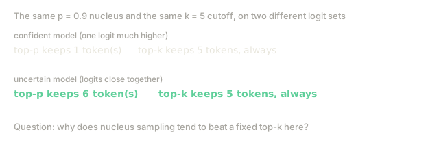
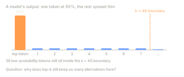
Top-k keeps the model from picking extremely unlikely tokens (typos, nonsense, anything sitting in the long tail of the vocabulary distribution). The problem is that k stays fixed no matter what the context looks like. When the model is confident and one token holds 95% of the probability, k = 40 still leaves 39 alternatives on the table. When the model is uncertain and probability is spread across a thousand tokens, that same k = 40 cuts off options that were actually plausible.
Top-p (Nucleus) Sampling
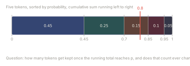
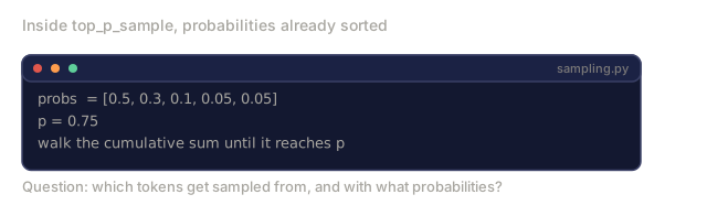
Top-p sampling adjusts the candidate set size on the fly. Instead of keeping a fixed number of tokens, it keeps the smallest set whose cumulative probability clears p.
Algorithm:
  1. Compute softmax probabilities for all V tokens
  2. Sort tokens by probability (descending)
  3. Find smallest k such that sum of top-k probabilities >= p
  4. Keep only those k tokens
  5. Renormalize and sample

p = 0.9:  keeps tokens covering 90% of probability mass
p = 1.0:  no filtering
p = 0.1:  very restrictive, nearly greedy
When the model is confident, nucleus sampling might keep only two or three tokens. When it's uncertain, it might keep two hundred. That adaptive behavior is exactly why nucleus sampling tends to beat top-k in practice.
Common combinations:
- Temperature 0.7 + top-p 0.9: good general-purpose setting
- Temperature 0.0 (greedy): best for deterministic tasks
- Temperature 1.0 + top-k 50: Fan et al. (2018) original paper setting
You can combine the two: apply top-k first, then top-p on whatever survives.
Reparameterization Trick (Used in VAEs)
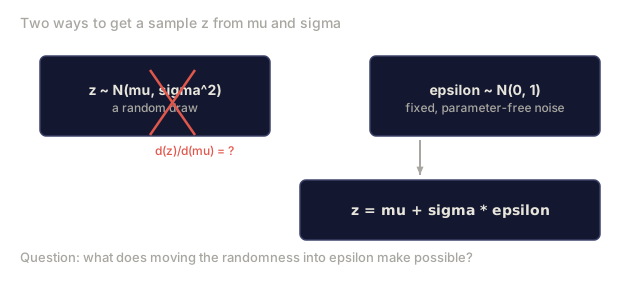
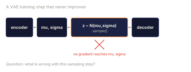
The reparameterization trick rewrites a random sample as a deterministic function of its parameters plus a separate, parameter-free noise term, so gradients can flow through what used to be a random draw. Variational autoencoders (VAEs) need exactly that: they learn by encoding inputs into a distribution in latent space, sampling from that distribution, and decoding the sample back, and without this trick you cannot backpropagate through the sampling step at all.
Standard sampling (not differentiable):
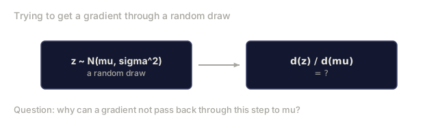
  z ~ N(mu, sigma^2)

  The randomness blocks gradient flow.
  d/d_mu [sample from N(mu, sigma^2)] = ???
The trick separates the randomness from the parameters:
Reparameterized sampling:
  epsilon ~ N(0, 1)          (fixed random noise, no parameters)
  z = mu + sigma * epsilon   (deterministic function of parameters)

  Now z is a deterministic, differentiable function of mu and sigma.
  d(z)/d(mu) = 1
  d(z)/d(sigma) = epsilon

  Gradients flow through mu and sigma.
This works because N(mu, sigma^2) has the same distribution as mu + sigma * N(0, 1). The key insight: move the randomness to a parameter-free source (epsilon), then express the sample as a differentiable transformation of the parameters.
In the VAE training loop:
- Encoder outputs mu and log(sigma^2) for each input
- Sample epsilon ~ N(0, 1)
- Compute z = mu + sigma * epsilon
- Decode z to reconstruct the input
- Backpropagate through steps 4, 3, 2, 1 (possible because step 3 is differentiable)
Without it, VAEs can't be trained with standard backpropagation at all. This one trick is what made VAEs practical in the first place.
Gumbel-Softmax (Differentiable Categorical Sampling)
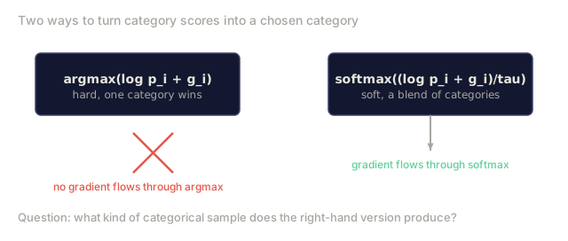
The reparameterization trick works for continuous distributions like the Gaussian. Discrete categorical distributions need a different approach: Gumbel-Softmax, a differentiable approximation to categorical sampling.
The Gumbel-Max trick (non-differentiable):
To sample from a categorical distribution with log-probabilities log(p_1), ..., log(p_k):
  1. Sample g_i ~ Gumbel(0, 1) for each category
     (g = -log(-log(u)), where u ~ Uniform(0, 1))
  2. Return argmax(log(p_i) + g_i)

This produces exact categorical samples.
Gumbel-Softmax (differentiable approximation):
Replace the hard argmax with a soft softmax:
  y_i = exp((log(p_i) + g_i) / tau) / sum(exp((log(p_j) + g_j) / tau))

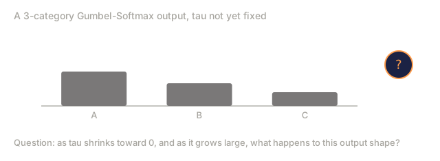
tau (temperature) controls the approximation:
  tau -> 0:  approaches a one-hot vector (hard categorical)
  tau -> inf: approaches uniform (1/k, 1/k, ..., 1/k)
  tau = 1.0: soft approximation
Gumbel-Softmax produces a continuous relaxation of a discrete sample. The output is a probability vector (soft one-hot) instead of a hard one-hot. Gradients flow through the softmax. During training, you can use the "straight-through" estimator: the hard argmax for the forward pass, the soft Gumbel-Softmax gradient for the backward pass.
Applications:
- Discrete latent variables in VAEs
- Neural architecture search (choosing discrete operations)
- Hard attention mechanisms
- Reinforcement learning with discrete actions
Stratified Sampling
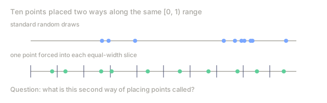
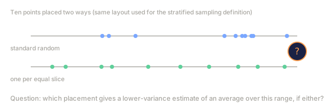
Standard Monte Carlo sampling can leave gaps in the sample space purely by chance. Stratified sampling forces even coverage instead: divide the space into strata and sample from each one.
Standard Monte Carlo:
  Sample N points uniformly from [0, 1]
  Some regions may have clusters, others gaps

Stratified sampling:
  Divide [0, 1] into N equal strata: [0, 1/N), [1/N, 2/N), ..., [(N-1)/N, 1)
  Sample one point uniformly within each stratum
  x_i = (i + u_i) / N   where u_i ~ Uniform(0, 1),  i = 0, ..., N-1
Stratified sampling always has lower or equal variance compared to standard Monte Carlo:
Var(stratified) <= Var(standard Monte Carlo)

The improvement is largest when f(x) varies smoothly.
For piecewise-constant functions, stratified sampling is exact.
Applications:
- Numerical integration (quasi-Monte Carlo)
- Training data splits (ensuring class balance in each fold)
- Importance sampling with stratification (combining both techniques)
- NeRF (Neural Radiance Fields) uses stratified sampling along camera rays
Connection to Diffusion Models
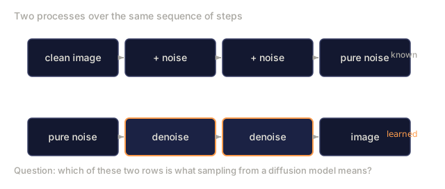
Diffusion models generate images through a sampling process. The forward process adds Gaussian noise to an image over T steps until it becomes pure noise. The reverse process learns to denoise, recovering the original image step by step.
Forward process (known):
  x_t = sqrt(alpha_t) * x_{t-1} + sqrt(1 - alpha_t) * epsilon
  where epsilon ~ N(0, I)

  After T steps: x_T ~ N(0, I)  (pure noise)

Reverse process (learned):
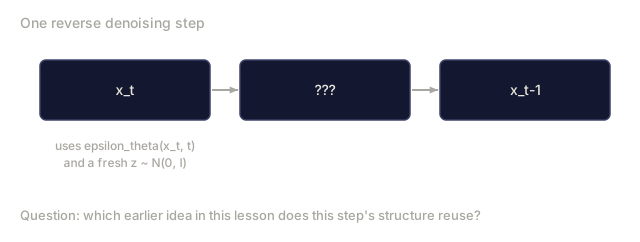
  x_{t-1} = (1/sqrt(alpha_t)) * (x_t - (1 - alpha_t)/sqrt(1 - alpha_bar_t) * epsilon_theta(x_t, t)) + sigma_t * z
  where z ~ N(0, I)

  Each denoising step is a sampling step.
The connection to the methods in this lesson:
- Each denoising step uses the reparameterization trick (sample noise, apply deterministic transform)
- The noise schedule {alpha_t} controls a form of temperature annealing
- Training uses Monte Carlo estimation to approximate the ELBO (evidence lower bound)
- Ancestral sampling in diffusion models is a Markov chain (each step depends only on the current state)
The entire image generation process is iterative sampling: start from noise, and at each step, sample a slightly less noisy version conditioned on the learned denoising model.

Build It
Step 1: Uniform and inverse CDF sampling
import math
import random

def sample_uniform(a, b):
    return a + (b - a) * random.random()

def sample_exponential_inverse_cdf(lam):
    u = random.random()
    return -math.log(u) / lam
Generate 10,000 exponential samples and verify the mean is 1/lambda.
Step 2: Rejection sampling
def rejection_sample(target_pdf, proposal_sample, proposal_pdf, M):
    while True:
        x = proposal_sample()
        u = random.random()
        if u < target_pdf(x) / (M * proposal_pdf(x)):
            return x
Use rejection sampling to draw from a truncated normal distribution. Verify the shape by histogramming the samples.
Step 3: Importance sampling
def importance_sampling_estimate(f, target_pdf, proposal_pdf, proposal_sample, n):
    total = 0
    for _ in range(n):
        x = proposal_sample()
        w = target_pdf(x) / proposal_pdf(x)
        total += f(x) * w
    return total / n
Estimate E[X^2] under a normal distribution using a uniform proposal. Compare to the known answer (mu^2 + sigma^2).
Step 4: Monte Carlo estimation of pi
def monte_carlo_pi(n):
    inside = 0
    for _ in range(n):
        x = random.uniform(-1, 1)
        y = random.uniform(-1, 1)
        if x*x + y*y <= 1:
            inside += 1
    return 4 * inside / n
Step 5: Metropolis-Hastings MCMC
def metropolis_hastings(target_log_pdf, proposal_sample, proposal_log_pdf, x0, n_samples, burn_in):
    samples = []
    x = x0
    for i in range(n_samples + burn_in):
        x_new = proposal_sample(x)
        log_alpha = (target_log_pdf(x_new) + proposal_log_pdf(x, x_new)
                     - target_log_pdf(x) - proposal_log_pdf(x_new, x))
        if math.log(random.random()) < log_alpha:
            x = x_new
        if i >= burn_in:
            samples.append(x)
    return samples
Sample from a bimodal distribution (mixture of two Gaussians). Visualize the chain's trajectory.
Step 6: Gibbs sampling
def gibbs_sampling_2d(conditional_x_given_y, conditional_y_given_x, x0, y0, n_samples, burn_in):
    x, y = x0, y0
    samples = []
    for i in range(n_samples + burn_in):
        x = conditional_x_given_y(y)
        y = conditional_y_given_x(x)
        if i >= burn_in:
            samples.append((x, y))
    return samples
Step 7: Temperature sampling
def softmax(logits):
    max_l = max(logits)
    exps = [math.exp(z - max_l) for z in logits]
    total = sum(exps)
    return [e / total for e in exps]

def temperature_sample(logits, temperature):
    scaled = [z / temperature for z in logits]
    probs = softmax(scaled)
    return sample_from_probs(probs)
Show how temperature changes the output distribution for a set of token logits.
Step 8: Top-k and top-p sampling
def top_k_sample(logits, k):
    indexed = sorted(enumerate(logits), key=lambda x: -x[1])
    top = indexed[:k]
    top_logits = [l for _, l in top]
    probs = softmax(top_logits)
    idx = sample_from_probs(probs)
    return top[idx][0]

def top_p_sample(logits, p):
    probs = softmax(logits)
    indexed = sorted(enumerate(probs), key=lambda x: -x[1])
    cumsum = 0
    selected = []
    for token_idx, prob in indexed:
        cumsum += prob
        selected.append((token_idx, prob))
        if cumsum >= p:
            break
    sel_probs = [pr for _, pr in selected]
    total = sum(sel_probs)
    sel_probs = [pr / total for pr in sel_probs]
    idx = sample_from_probs(sel_probs)
    return selected[idx][0]
Step 9: Reparameterization trick
def reparam_sample(mu, sigma):
    epsilon = random.gauss(0, 1)
    return mu + sigma * epsilon

def reparam_gradient(mu, sigma, epsilon):
    dz_dmu = 1.0
    dz_dsigma = epsilon
    return dz_dmu, dz_dsigma
Demonstrate that gradients flow through the reparameterized sample but not through direct sampling.
Step 10: Gumbel-Softmax
def gumbel_sample():
    u = random.random()
    return -math.log(-math.log(u))

def gumbel_softmax(logits, temperature):
    gumbels = [math.log(p) + gumbel_sample() for p in logits]
    return softmax([g / temperature for g in gumbels])
Show how decreasing temperature makes the output approach a one-hot vector.
Full implementations with all visualizations are in code/sampling.py.
Use It
Here's the production version, with NumPy and SciPy doing the heavy lifting:
import numpy as np

rng = np.random.default_rng(42)

exponential_samples = rng.exponential(scale=2.0, size=10000)
print(f"Exponential mean: {exponential_samples.mean():.4f} (expected 2.0)")

from scipy import stats
normal = stats.norm(loc=0, scale=1)
print(f"CDF at 1.96: {normal.cdf(1.96):.4f}")
print(f"Inverse CDF at 0.975: {normal.ppf(0.975):.4f}")

logits = np.array([2.0, 1.0, 0.5, 0.1, -1.0])
temperature = 0.7
scaled = logits / temperature
probs = np.exp(scaled - scaled.max()) / np.exp(scaled - scaled.max()).sum()
token = rng.choice(len(logits), p=probs)
print(f"Sampled token index: {token}")
For MCMC at scale, use dedicated libraries:
- PyMC: full Bayesian modeling with NUTS (adaptive HMC)
- emcee: ensemble MCMC sampler
- NumPyro/JAX: GPU-accelerated MCMC
You built these from scratch. Now you know what the library calls are doing.
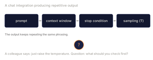
In production you will not write your own Metropolis-Hastings sampler or invert a CDF by hand. You will set two numbers, temperature and top-p, on an API call and move on. But the time I spent building rejection sampling and MCMC from scratch paid off in a different way: when an LLM integration starts producing weird, repetitive, or degenerate output, "just raise the temperature" is usually the wrong fix. The real bug is almost always upstream: a bad prompt, a broken stop condition, a context window doing something you didn't expect, and temperature is being asked to paper over it. Once you've built nucleus sampling from the algorithm up, you stop treating it as a vibe slider and start treating it for what it is: a precise statement about how much probability mass you're willing to keep. That makes it a debugging tool first, a creativity dial second.
Exercises
-
Implement inverse CDF sampling for the Cauchy distribution. The CDF is F(x) = 0.5 + arctan(x)/pi. Generate 10,000 samples and plot the histogram against the true PDF. Notice the heavy tails (extreme values far from center).
-
Use rejection sampling to generate samples from a Beta(2, 5) distribution using a Uniform(0, 1) proposal. Plot the accepted samples against the true Beta PDF. What is the theoretical acceptance rate?
-
Estimate the integral of sin(x) from 0 to pi using Monte Carlo with 1,000, 10,000, and 100,000 samples. Compare the error at each level. Verify that the error scales as O(1/sqrt(N)).
-
Implement Metropolis-Hastings to sample from a 2D distribution p(x, y) proportional to exp(-(x^2 * y^2 + x^2 + y^2 - 8x - 8y) / 2). Plot the samples and the chain trajectory. Experiment with different proposal standard deviations.
-
Build a complete text generation demo: given a vocabulary of 10 words with logits, generate sequences of 20 tokens using (a) greedy, (b) temperature=0.7, (c) top-k=3, (d) top-p=0.9. Compare the diversity of outputs across 5 runs.
Key Terms
| Term | What people say | What it actually means |
|---|---|---|
| Sampling | "Drawing random values" | Generating values according to a probability distribution. The mechanism behind all generative AI |
| Uniform distribution | "All equally likely" | Every value in [a, b] has equal probability density 1/(b-a). The starting point for all sampling methods |
| Inverse CDF | "Probability transform" | F_inverse(U) converts a uniform sample into a sample from any distribution with known CDF. Exact and efficient |
| Rejection sampling | "Propose and accept/reject" | Generate from a simple proposal, accept with probability proportional to target/proposal ratio. Exact but wastes samples |
| Importance sampling | "Reweight samples" | Estimate expectations under p(x) using samples from q(x) by weighting each sample by p(x)/q(x). Core to PPO in RL |
| Monte Carlo | "Average random samples" | Approximate integrals as sample averages. Error O(1/sqrt(N)) regardless of dimension |
| MCMC | "Random walk that converges" | Construct a Markov chain whose stationary distribution is the target. Metropolis-Hastings is the foundational algorithm |
| Metropolis-Hastings | "Accept uphill, sometimes downhill" | Propose moves, accept based on density ratio. Detailed balance ensures convergence to target distribution |
| Gibbs sampling | "One variable at a time" | Update each variable from its conditional distribution holding others fixed. 100% acceptance rate |
| Temperature | "Confidence knob" | Divides logits by T before softmax. T<1 sharpens (more confident), T>1 flattens (more diverse) |
| Top-k sampling | "Keep the k best" | Zero out all but the k highest-probability tokens, renormalize, sample. Fixed candidate set size |
| Nucleus sampling (top-p) | "Keep the probable ones" | Keep the smallest set of tokens whose cumulative probability exceeds p. Adaptive candidate set size |
| Reparameterization trick | "Move randomness outside" | Write z = mu + sigma * epsilon where epsilon ~ N(0,1). Makes sampling differentiable. Essential for VAE training |
| Gumbel-Softmax | "Soft categorical sampling" | Differentiable approximation to categorical sampling using Gumbel noise + softmax with temperature |
| Stratified sampling | "Forced coverage" | Divide sample space into strata, sample from each. Always lower variance than naive Monte Carlo |
| Burn-in | "Warm-up period" | Initial MCMC samples discarded before the chain reaches its stationary distribution |
| Detailed balance | "Reversibility condition" | p(x) * T(x->y) = p(y) * T(y->x). Sufficient condition for p to be the stationary distribution of a Markov chain |
| Diffusion sampling | "Iterative denoising" | Generate data by starting from noise and applying learned denoising steps. Each step is a conditional sampling operation |
Further Reading
- Holbrook (2023): The Metropolis-Hastings Algorithm - detailed tutorial on MCMC foundations
- Jang, Gu, Poole (2017): Categorical Reparameterization with Gumbel-Softmax - original Gumbel-Softmax paper
- Holtzman et al. (2020): The Curious Case of Neural Text Degeneration - nucleus (top-p) sampling paper
- Kingma & Welling (2014): Auto-Encoding Variational Bayes - VAE paper introducing the reparameterization trick
- Ho, Jain, Abbeel (2020): Denoising Diffusion Probabilistic Models - DDPM connects sampling to image generation
Code
- sampling.py (python, 749 lines)