GPT — Causal Language Modeling
BERT sees both sides of a token. GPT sees the tokens before it. The triangle mask is one line of code, and a lot of modern AI rests on it.
Learning Objectives
- Explain how the causal mask lets one forward pass produce a next-token prediction at every position in parallel.
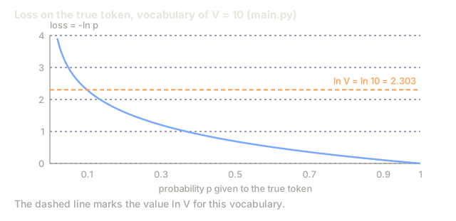
- Compute the shift-by-one cross-entropy loss and compare it against the random baseline ln V.
- Implement greedy, temperature, top-k, top-p and min-p sampling and say when each one fits.
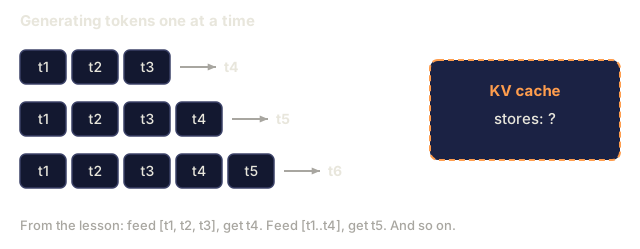
- Explain why GPT inference is serial even though training is parallel, and what the KV cache saves.
The Problem
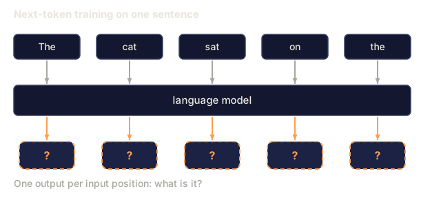
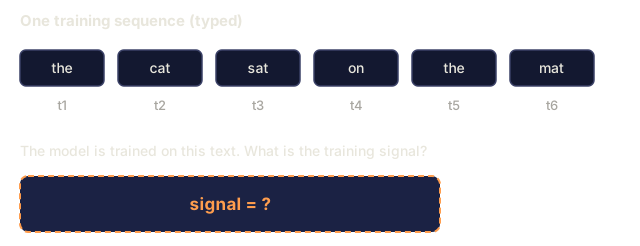
A language model is a function that takes the first t-1 tokens and returns a probability distribution over token t. Train on that signal, next-token prediction, and you get a model that generates text one token at a time.
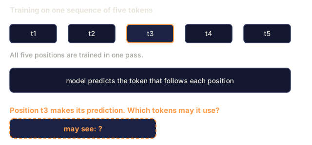
To train on a whole sequence in parallel, each position's prediction has to depend on earlier positions alone. If a position could see later tokens, the model would be reading the answer off the page.
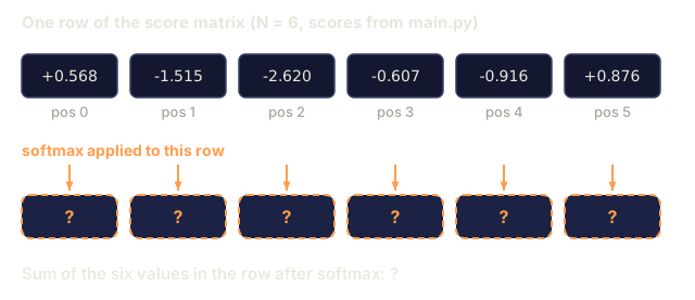
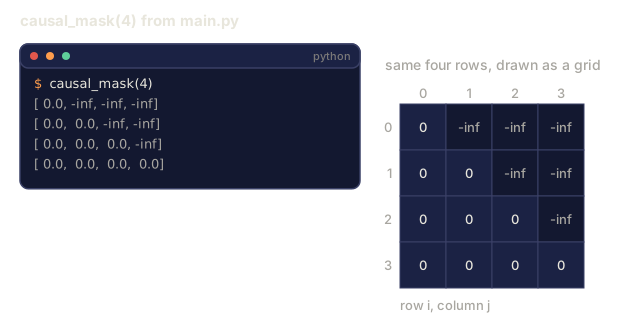
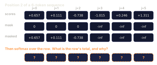
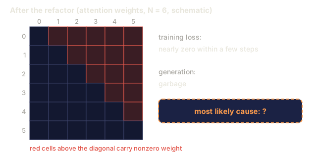
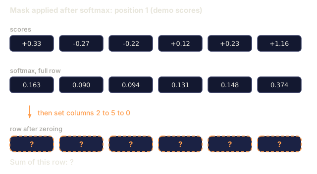
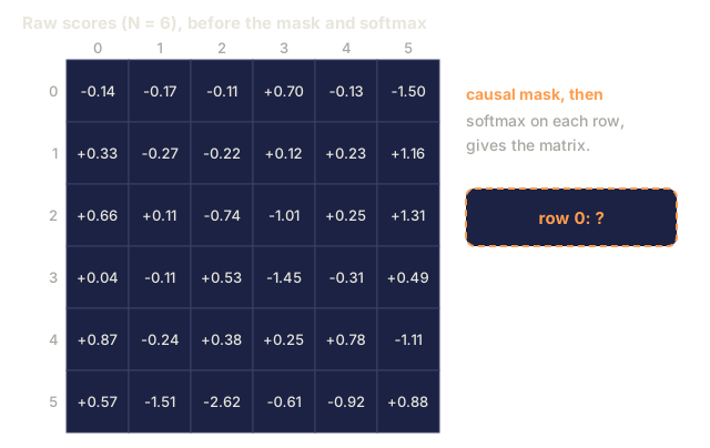
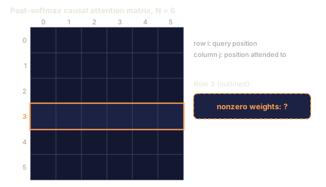
The causal mask enforces that. It is an upper-triangular matrix of -inf values added to the attention scores before softmax. After softmax those positions become 0, so each position attends to itself and earlier positions. Apply the mask once to the whole sequence and one forward pass gives you N parallel next-token predictions.
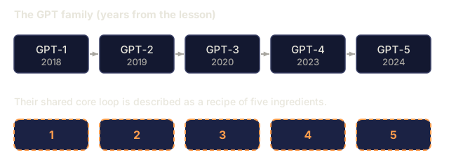
GPT-1 (2018), GPT-2 (2019), GPT-3 (2020), GPT-4 (2023), GPT-5 (2024), Claude, Llama, Qwen, Mistral, DeepSeek and Kimi are decoder-only causal transformers with the same core loop. What differs is size, data quality, and RLHF.
The Concept

The mask
The causal mask is an N × N matrix, for a sequence of length N, that blocks each position from attending to later ones:
M[i, j] = 0       if j <= i
M[i, j] = -inf    if j > i
Add M to the raw attention scores before softmax. Since exp(-inf) = 0, masked positions get zero weight, and each row of the attention matrix is a probability distribution over previous positions (and the current one).
Implementation cost: one line. code/main.py builds it with a nested list comprehension, and in PyTorch it is one torch.tril() call. Time to compute: nanoseconds. Impact on the field: enormous.
Parallel training, serial inference
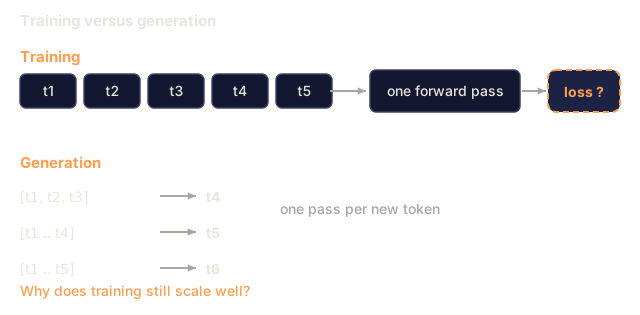
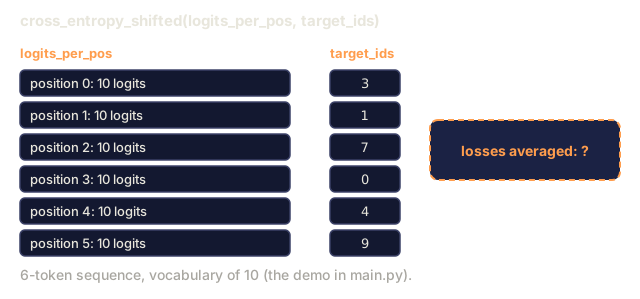
Training runs the whole (N, d_model) sequence through one forward pass, computes N cross-entropy losses (one per position), averages them, and backpropagates. The work is parallel along the sequence, which is why GPT training scales: a batch of 1M tokens goes through in one GPU pass.
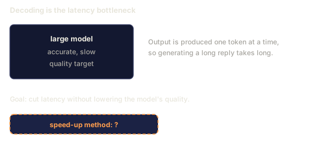
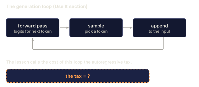
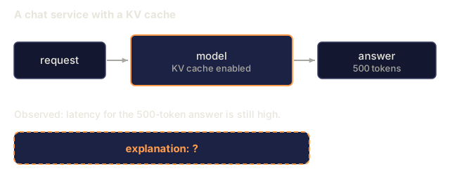
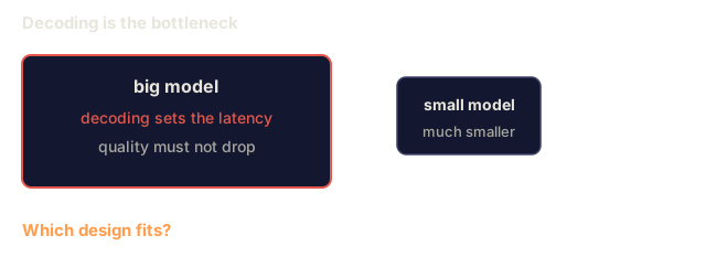
Inference is token by token. Feed [t1, t2, t3], get t4. Feed [t1, t2, t3, t4], get t5. Feed [t1, t2, t3, t4, t5], get t6. The KV cache (Lesson 12) saves the hidden states of t1…tn so you don't recompute them at each step, but serial depth at inference still equals output length. That is the autoregressive tax, and it is why decoding is the latency bottleneck for LLMs.
The loss: shift by one
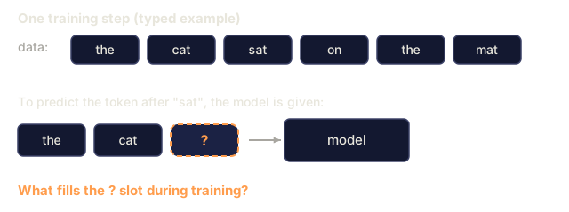
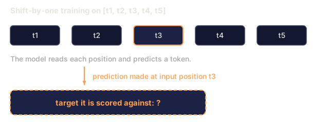
Given tokens [t1, t2, t3, t4]:
- Input:
[t1, t2, t3] - Targets:
[t2, t3, t4]
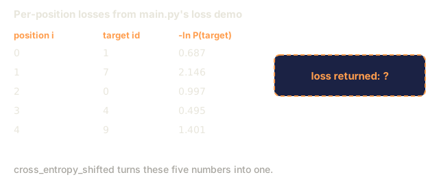
At each position i, compute -log P(target_i | inputs[:i+1]). Average these and you have the cross-entropy for the whole sequence.
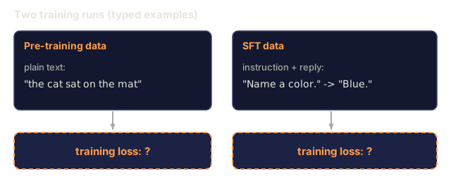
Pre-training, fine-tuning and SFT all use this loss. The data changes, the loss stays the same.
Decoding strategies
After training, the sampling choice matters more than most people expect.
| Method | What it does | When to use |
|---|---|---|
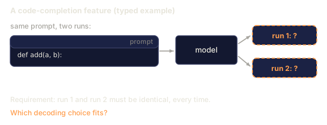
| Greedy | Argmax every step | Deterministic tasks, code completion |
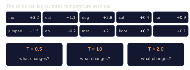
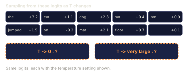
| Temperature | Divide logits by T, sample | Creative tasks, higher T = more diversity |
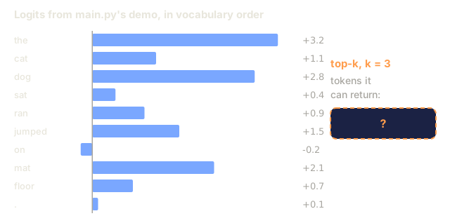
| Top-k | Sample from top-k tokens only | Kills low-probability tails |
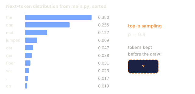
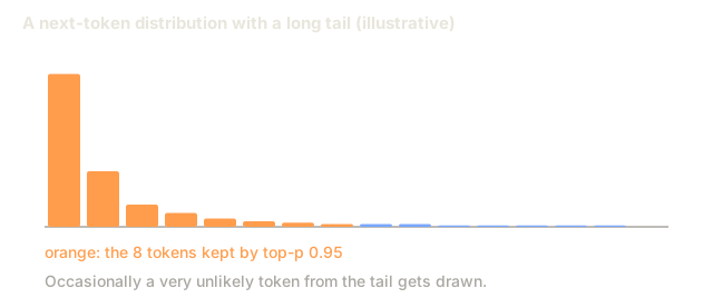
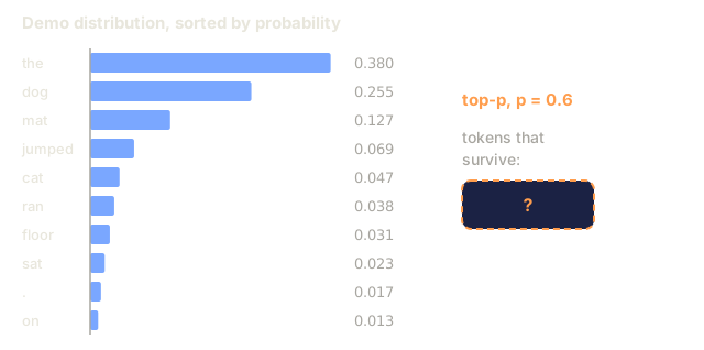
| Top-p (nucleus) | Sample from smallest set with cumulative prob ≥ p | 2020+ default; adapts to distribution shape |
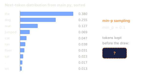
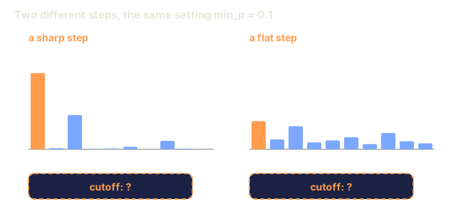
| Min-p | Keep tokens with p >= min_p * max_p | 2024+; better at rejecting long tails than top-p |
| Speculative decoding | Draft model proposes N tokens, big model verifies | 2–3× latency reduction at same quality |
code/main.py implements the first five rows (greedy, temperature, top-k, top-p, min-p). Speculative decoding is described here but not implemented in the file, and neither is beam search (Exercise 2).
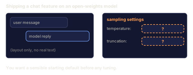
In 2026, min-p with temperature 0.7 is a reasonable default for open-weights models. Speculative decoding is table stakes for a production inference stack.
What made the "GPT recipe" work
- Decoder-only. No encoder overhead. One pass of attention + FFN per layer.
- Scaling. 124M → 1.5B → 175B → trillions. Chinchilla scaling laws (Lesson 13) tell you how to spend compute.
- In-context learning. Emerged around 6B–13B. The model can follow few-shot examples without fine-tuning.
- RLHF. Post-training on human preferences turned raw pretrained text into chat assistants.
- Pre-norm + RoPE + SwiGLU. Stable training at scale.
The core architecture has changed little since GPT-2. The interesting progress has come from data, scale, and post-training.
Build It
Step 1: the causal mask
See code/main.py. It fits in one line:
def causal_mask(n):
    return [[0.0 if j <= i else float("-inf") for j in range(n)] for i in range(n)]
Add it to the attention scores before softmax. That is the mechanism.
Step 2: a 2-layer GPT-ish model (design sketch, not in main.py)
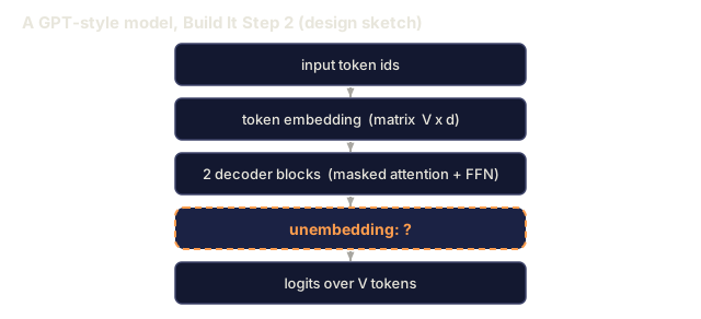
code/main.py has no model at all. It stands in random Gaussian scores for the attention matrix and random Gaussian logits for the output, which is enough to demonstrate the mask, the loss and the samplers. A real version would stack two decoder blocks (masked self-attention + FFN, no cross-attention), with a token embedding, a positional encoding, and an unembedding tied to the token embedding matrix (a standard trick since GPT-2).
Step 3: next-token prediction, end to end
On a 10-token toy vocab, take random Gaussian logits at each position, boost the true next token by +2.0 to mimic a slightly trained model, and compute cross-entropy loss against the shift-by-one target. There is no gradient step here. Treat it as a forward-pass sanity check.
Step 4: sampling
Implement greedy, temperature, top-k, top-p and min-p. Run each on a fixed prompt and compare the outputs. Each sampling function in code/main.py is short (top-k is about 8 lines, top-p and min-p 15 to 20 each).
Use It
PyTorch, 2026 idiom:
from transformers import AutoModelForCausalLM, AutoTokenizer
model = AutoModelForCausalLM.from_pretrained("meta-llama/Llama-3.2-3B-Instruct")
tok = AutoTokenizer.from_pretrained("meta-llama/Llama-3.2-3B-Instruct")

prompt = "Attention is all you need because"
inputs = tok(prompt, return_tensors="pt")
out = model.generate(
    **inputs,
    max_new_tokens=64,
    temperature=0.7,
    top_p=0.9,
    do_sample=True,
)
print(tok.decode(out[0]))
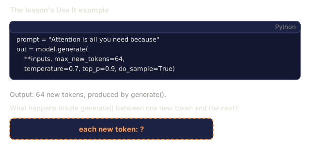
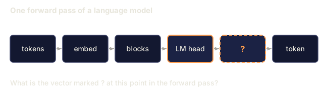
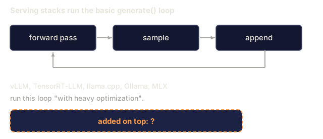
Under the hood, generate() runs the forward pass, pulls the final-position logits, samples the next token, appends it, and repeats. Production LLM inference stacks (vLLM, TensorRT-LLM, llama.cpp, Ollama, MLX) run the same loop with heavy optimization: batched prefill, continuous batching, KV cache paging, speculative decoding.
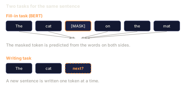
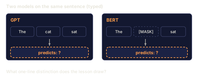
GPT vs BERT, one line each: GPT predicts P(x_t | x_{<t}). BERT predicts P(x_masked | x_unmasked). The loss determines whether the model can generate.
Ship It
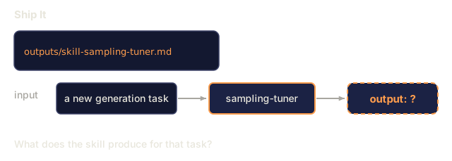
The sampling-tuner skill lives in outputs/skill-sampling-tuner.md. It picks sampling parameters for a new generation task and flags when deterministic decoding is required.
I'd run main.py and read the post-softmax matrix first. The mask is one line, but what to look at is the zeros above the diagonal and the fact that each row is still a distribution over positions 0..i. Predict row 0 before you print it: it has only one unmasked position, so all of its weight lands on position 0.
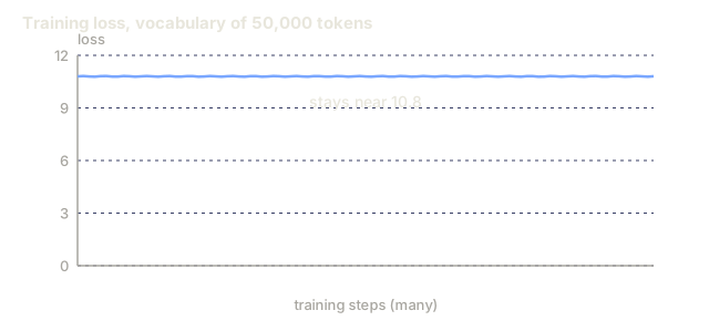
My bet is that the loss demo is the most useful output in the file. It prints the loss for slightly boosted logits, the loss for random logits, and the random baseline ln V for a 10-token vocab. A loss at ln V means the model is doing no better than guessing uniformly, so I'd compare a training loss against that number first.
For sampling, I'd start with min-p and temperature 0.7, the default suggested under the decoding table, then run the sampling demo to see where the strategies disagree on one fixed distribution. Get a feel for that on the toy before tuning on a real model.
Exercises
- Easy. Run
code/main.pyand check by eye that the printed causal attention matrix is lower-triangular after softmax (the demo only prints it, so add anassertif you want a hard check). Spot-check: row 3 should have weights only in columns 0–3. - Medium. Implement beam search with width 4 (not in
main.py, you write it). Compare perplexity of beam-4 vs greedy on 10 short prompts. Does beam win? (Hint: it tends to for translation, not for open-ended chat.) - Hard. Implement speculative decoding (also not in
main.py): use a tiny 2-layer model as the draft and a 6-layer model as the verifier. Measure wall-clock speedup on 100 completions of length 64. Confirm the outputs match greedy decoding of the verifier.
Key Terms
| Term | What people say | What it actually means |
|---|---|---|
| Causal mask | "The triangle" | Upper-triangular -inf matrix added to attention scores so position i sees positions up to and including i. |
| Next-token prediction | "The loss" | Cross-entropy of the model's distribution against the true next token at each position. |
| Autoregressive | "Generate one at a time" | Feed output back in as input. Training is parallel across positions, generation is serial. |
| Logits | "Pre-softmax scores" | Raw output of the LM head before softmax. Sampling happens on these. |
| Temperature | "Creativity knob" | Divide logits by T. T→0 approaches greedy, T→∞ approaches uniform. |
| Top-p | "Nucleus sampling" | Truncate the distribution to the smallest set summing to ≥p, then sample from what remains. |
| Min-p | "Better than top-p" | Keep tokens where p ≥ min_p × max_p, so the cutoff adapts to how sharp the distribution is. |
| Speculative decoding | "Draft + verify" | A cheap model proposes N tokens and the big model verifies them in parallel. Described in this lesson, not implemented in main.py. |
| Teacher forcing | "Training trick" | During training, feed the true previous token instead of the model's prediction. Standard for seq2seq LMs. |
Further Reading
- Radford et al. (2018). Improving Language Understanding by Generative Pre-Training: GPT-1.
- Radford et al. (2019). Language Models are Unsupervised Multitask Learners: GPT-2.
- Brown et al. (2020). Language Models are Few-Shot Learners: GPT-3 and in-context learning.
- Leviathan, Kalman, Matias (2023). Fast Inference from Transformers via Speculative Decoding: spec decoding paper.
- HuggingFace
modeling_llama.py: canonical causal-LM reference code.
Code
- main.py (python, 179 lines)