Pre-Training a Mini GPT (124M Parameters)
GPT-2 Small has 124 million parameters: 12 transformer layers, 12 attention heads, 768-dimensional embeddings. You can train it from scratch on a single GPU in a few hours. Few people do. They pull a pre-trained checkpoint and build on top of it. But if you haven't trained one yourself, you're building products on a model you only half understand.
Learning Objectives
- Implement the full GPT-2 architecture (124M parameters) from scratch: token embeddings, positional embeddings, transformer blocks, and the language model head
- Train a GPT model on a text corpus using next-token prediction with cross-entropy loss
- Implement autoregressive text generation with temperature sampling, then extend it with top-k/top-p filtering in the exercises
- Monitor training loss curves and validate that the model learns coherent language patterns
- Estimate parameter counts and KV cache memory for the GPT-2 family and larger models
The Problem
You know what a transformer is. You've read the diagrams, you can recite "attention is all you need", and you can draw a box labeled "Multi-Head Attention" on a whiteboard. None of that tells you what happens when a model generates text.
GPT-2 Small has 124,438,272 parameters (with weight tying). A training loop set each one: forward pass, loss, backward pass, weight update. The shape is twelve transformer blocks, twelve attention heads per block, a 768-dimensional embedding space, and a vocabulary of 50,257 tokens. To generate a token, the model runs one chain of matrix multiplications that turns a sequence of token IDs into a probability distribution over the next token.
If you haven't built this yourself, the model is a black box. You can call the API and you can fine-tune, but when it hallucinates, repeats itself, or ignores an instruction, you have no mental model for why.
So we build GPT-2 Small from scratch, in numpy instead of PyTorch. Every matrix multiplication stays visible and the gradient code is yours to read. By the end you'll see how 124 million numbers turn into a prediction of the next word.
The Concept
The GPT Architecture
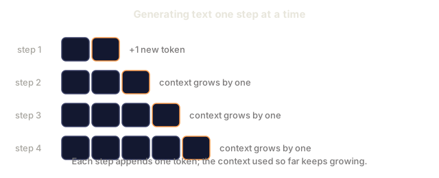
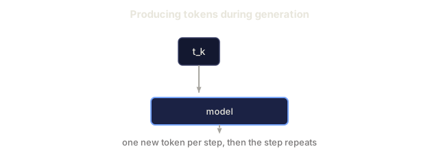
GPT is an autoregressive language model: it generates one token at a time, each conditioned on all the tokens before it. The architecture is a stack of transformer decoder blocks. Here is the full path from token IDs to next-token probabilities:
- Token IDs come in. Shape: (batch_size, seq_len).
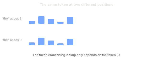
- Token embedding lookup. Each ID maps to a 768-dimensional vector. Shape: (batch_size, seq_len, 768).
- Position embedding lookup. Each position (0, 1, 2, ...) maps to a 768-dimensional vector. Same shape.
- Add token embeddings + position embeddings.
- Pass through 12 transformer blocks.
- Final layer normalization.
- Linear projection to vocabulary size. Shape: (batch_size, seq_len, vocab_size).
- Softmax to get probabilities.
That is the whole model. There are no convolutions and no recurrence, just embeddings, attention, feedforward networks, and layer norms, stacked 12 times.

The Transformer Block
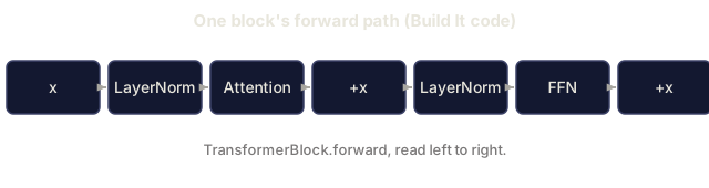
All 12 blocks follow the same pre-norm pattern. GPT-2 normalizes before each sublayer, where the original transformer normalized after:
- LayerNorm
- Multi-Head Self-Attention
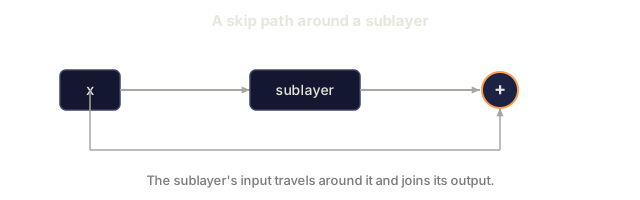
- Residual connection (add input back)
- LayerNorm
- Feed-Forward Network (MLP)
- Residual connection (add input back)
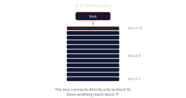
The residual connections carry a lot of weight. Without them, gradients tend to vanish before they reach block 1 during backpropagation. With them, gradients flow from the loss back to earlier layers through the skip path, which is why you can stack 12, 32, or 96 blocks (GPT-4 is rumored to use 120).
Attention: The Core Mechanism
Self-attention lets each token look at the earlier tokens and decide how much weight each one gets. For each token position, compute three vectors from the input:
- Query (Q): "What am I looking for?"
- Key (K): "What do I contain?"
- Value (V): "What information do I carry?"
Q = input @ W_q    (768 -> 768)
K = input @ W_k    (768 -> 768)
V = input @ W_v    (768 -> 768)

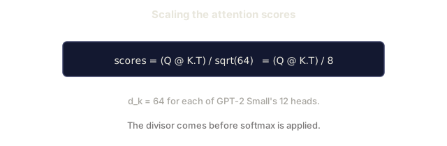
attention_scores = Q @ K^T / sqrt(d_k)
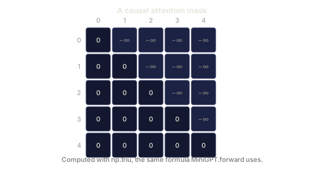
attention_scores = mask(attention_scores)   # causal mask: -inf for future positions
attention_weights = softmax(attention_scores)
output = attention_weights @ V
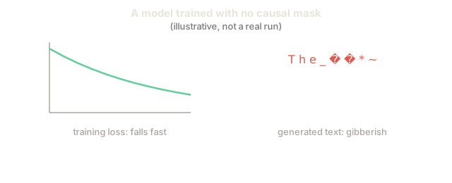
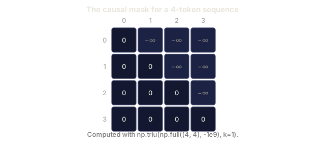
The causal mask is what makes GPT autoregressive. Position 5 attends to positions 0-5 and nothing after. Without the mask, the model could cheat during training by reading the future tokens it is supposed to predict.
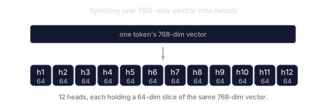
Multi-head attention splits the 768-dimensional space into 12 heads of 64 dimensions each, and each head can learn a different attention pattern. One might track syntax (subject-verb agreement), another semantic similarity, another nearby words. The 12 outputs are concatenated and projected back to 768 dimensions.

The division by sqrt(d_k) (sqrt(64) = 8) is a scaling step from the original "Attention Is All You Need" paper. Without it, dot products grow large in high dimensions and push softmax into regions where gradients are nearly zero.
KV Cache: Why Inference Is Fast
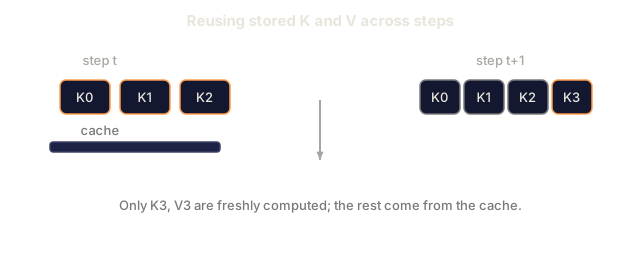
Training processes the entire sequence at once. Inference generates one token at a time, and without optimization, generating token N means recomputing attention for all N-1 previous tokens. That is O(N^2) per generated token, or O(N^3) total for a sequence of length N.
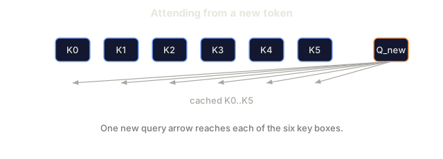
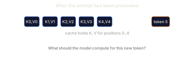
The KV cache fixes this. After computing K and V for each token, store them. To generate token N+1, compute Q for the new token and look up the cached K and V for the earlier ones. That cuts the K and V computation per token from O(N) to O(1). The attention scores are still O(N) because the new token attends to every previous position, but the redundant matrix multiplications on the input are gone.
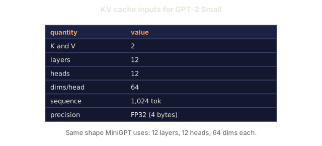
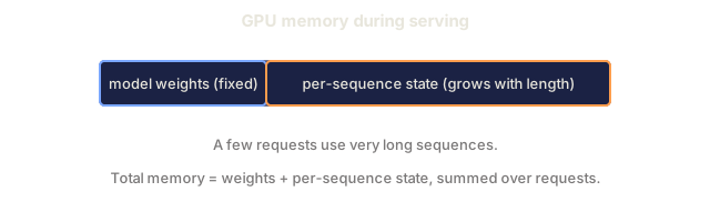
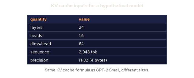
For GPT-2 with 12 layers and 12 heads, the KV cache stores 2 (K + V) x 12 layers x 12 heads x 64 dims = 18,432 values per token. For a 1024-token sequence, that is about 75MB in FP32. Llama 3 405B has 126 layers, and its KV cache for a single long sequence can exceed 10GB. That is one reason long-context inference is memory-bound.
Prefill vs Decode: Two Phases of Inference
Inference on a prompt runs in two phases.
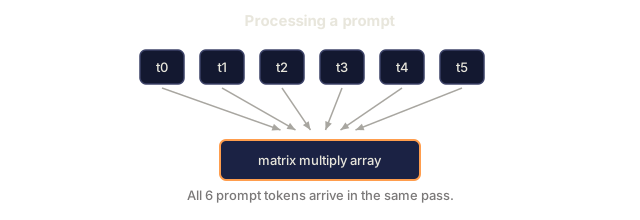
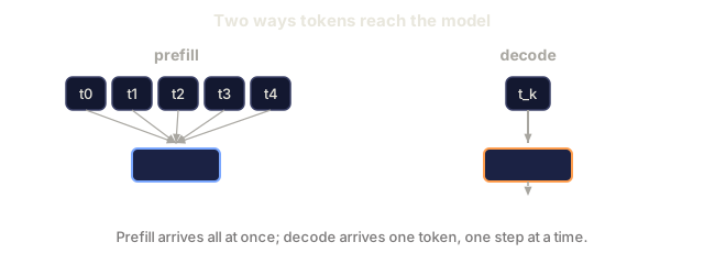
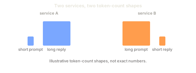
Prefill processes your entire prompt in parallel. All tokens are known, so attention for every position is computed at once. This phase is compute-bound: the GPU spends its time on matrix multiplications. For a 1000-token prompt on an A100, prefill takes roughly 20-50ms.
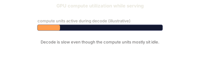
Decode generates tokens one at a time, each depending on all the previous ones. This phase is memory-bound. The bottleneck is reading the model weights and KV cache from GPU memory, so the compute cores sit mostly idle waiting on memory. For GPT-2, a decode step takes about the same time whatever the matmuls cost in FLOPs, because memory bandwidth is the constraint.
The split matters in production. Prefill throughput scales with GPU compute (more FLOPS = faster prefill). Decode throughput scales with memory bandwidth (faster memory = faster decode). That is why NVIDIA's H100 focused on memory bandwidth improvements over the A100, since it directly speeds up token generation.

The Training Loop
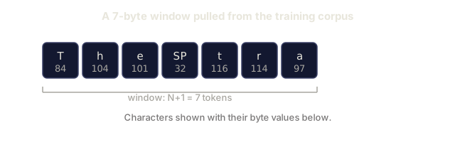
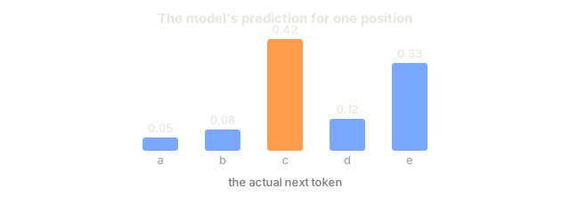
Training an LLM is next-token prediction: given tokens [0, 1, 2, ..., N-1], predict tokens [1, 2, 3, ..., N]. The loss is cross-entropy between the model's predicted distribution and the actual next token.
One training step:
- Forward pass: Run the batch through all 12 blocks. Get logits (pre-softmax scores) for each position.
- Compute loss: Cross-entropy between logits and target tokens (the input shifted by one position).
- Backward pass: Compute gradients for all 124M parameters using backpropagation.
- Optimizer step: Update weights. GPT-2 uses Adam with learning rate warmup and cosine decay.
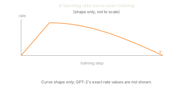
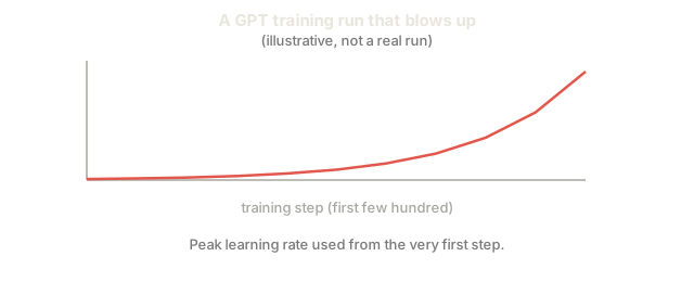
The learning rate schedule matters more than it looks. GPT-2 warms up from 0 to the peak learning rate over the first 2,000 steps, then decays along a cosine curve. Starting at a high rate can make the model diverge, and holding a high rate makes it oscillate late in training. Warmup then decay is the pattern used by every major LLM.
GPT-2 Small: The Numbers
| Component | Shape | Parameters |
|---|---|---|
| Token embeddings | (50257, 768) | 38,597,376 |
| Position embeddings | (1024, 768) | 786,432 |
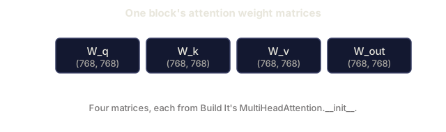
| Per-block attention (W_q, W_k, W_v, W_out) | 4 x (768, 768) | 2,359,296 |
| Per-block FFN (up + down) | (768, 3072) + (3072, 768) | 4,718,592 |
| Per-block LayerNorms (2x) | 2 x 768 x 2 | 3,072 |
| Final LayerNorm | 768 x 2 | 1,536 |
| Total per block | 7,080,960 | |
| Total (12 blocks) | 85,054,464 + 39,383,808 = 124,438,272 |
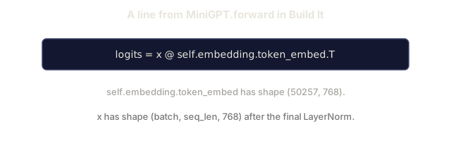
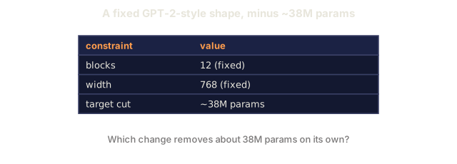
The output projection (logits head) shares weights with the token embedding matrix. This is called weight tying. It cuts the parameter count by 38M and improves performance, because the model uses one representation space for both input and output.


Build It
Step 1: Embedding Layer
Token embeddings map each of the 50,257 tokens to a 768-dimensional vector. Position embeddings say where each token sits in the sequence. The two are summed.
import numpy as np

class Embedding:
    def __init__(self, vocab_size, embed_dim, max_seq_len):
        self.token_embed = np.random.randn(vocab_size, embed_dim) * 0.02
        self.pos_embed = np.random.randn(max_seq_len, embed_dim) * 0.02

    def forward(self, token_ids):
        seq_len = token_ids.shape[-1]
        tok_emb = self.token_embed[token_ids]
        pos_emb = self.pos_embed[:seq_len]
        return tok_emb + pos_emb
The 0.02 standard deviation for initialization comes from the GPT-2 paper. Too large and the initial forward passes produce extreme values that destabilize training. Too small and the initial outputs barely differ across inputs, so the early gradients carry little information.
Step 2: Self-Attention with Causal Mask
Single-head attention first. The causal mask sets future positions to negative infinity before softmax, so each position attends only to itself and earlier positions.
def attention(Q, K, V, mask=None):
    d_k = Q.shape[-1]
    scores = Q @ K.transpose(0, -1, -2 if Q.ndim == 4 else 1) / np.sqrt(d_k)
    if mask is not None:
        scores = scores + mask
    weights = np.exp(scores - scores.max(axis=-1, keepdims=True))
    weights = weights / weights.sum(axis=-1, keepdims=True)
    return weights @ V
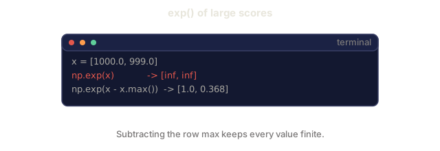
The softmax subtracts the maximum before exponentiating, because exp of a large number overflows to infinity. The output is unchanged, since softmax(x - c) = softmax(x) for a constant c.
Step 3: Multi-Head Attention
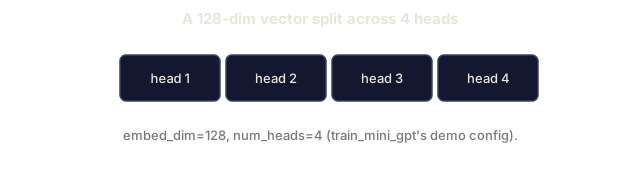
Split the 768-dimensional input into 12 heads of 64 dimensions, run attention in each head independently, concatenate the results, and project back to 768.
class MultiHeadAttention:
    def __init__(self, embed_dim, num_heads):
        self.num_heads = num_heads
        self.head_dim = embed_dim // num_heads
        self.W_q = np.random.randn(embed_dim, embed_dim) * 0.02
        self.W_k = np.random.randn(embed_dim, embed_dim) * 0.02
        self.W_v = np.random.randn(embed_dim, embed_dim) * 0.02
        self.W_out = np.random.randn(embed_dim, embed_dim) * 0.02

    def forward(self, x, mask=None):
        batch, seq_len, d = x.shape
        Q = (x @ self.W_q).reshape(batch, seq_len, self.num_heads, self.head_dim).transpose(0, 2, 1, 3)
        K = (x @ self.W_k).reshape(batch, seq_len, self.num_heads, self.head_dim).transpose(0, 2, 1, 3)
        V = (x @ self.W_v).reshape(batch, seq_len, self.num_heads, self.head_dim).transpose(0, 2, 1, 3)

        scores = Q @ K.transpose(0, 1, 3, 2) / np.sqrt(self.head_dim)
        if mask is not None:
            scores = scores + mask
        weights = np.exp(scores - scores.max(axis=-1, keepdims=True))
        weights = weights / weights.sum(axis=-1, keepdims=True)
        attn_out = weights @ V

        attn_out = attn_out.transpose(0, 2, 1, 3).reshape(batch, seq_len, d)
        return attn_out @ self.W_out
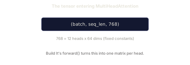
The reshape-transpose-reshape dance is the most confusing part of multi-head attention. The (batch, seq_len, 768) tensor becomes (batch, seq_len, 12, 64), then (batch, 12, seq_len, 64), so each head has its own (seq_len, 64) matrix to run attention on. Afterward the steps reverse, ending back at (batch, seq_len, 768).
Step 4: Transformer Block
One complete transformer block: LayerNorm, multi-head attention with residual, LayerNorm, feedforward with residual.
class LayerNorm:
    def __init__(self, dim, eps=1e-5):
        self.gamma = np.ones(dim)
        self.beta = np.zeros(dim)
        self.eps = eps

    def forward(self, x):
        mean = x.mean(axis=-1, keepdims=True)
        var = x.var(axis=-1, keepdims=True)
        return self.gamma * (x - mean) / np.sqrt(var + self.eps) + self.beta


class FeedForward:
    def __init__(self, embed_dim, ff_dim):
        self.W1 = np.random.randn(embed_dim, ff_dim) * 0.02
        self.b1 = np.zeros(ff_dim)
        self.W2 = np.random.randn(ff_dim, embed_dim) * 0.02
        self.b2 = np.zeros(embed_dim)

    def forward(self, x):
        h = x @ self.W1 + self.b1
        h = np.maximum(0, h)  # GELU approximation: ReLU for simplicity
        return h @ self.W2 + self.b2


class TransformerBlock:
    def __init__(self, embed_dim, num_heads, ff_dim):
        self.ln1 = LayerNorm(embed_dim)
        self.attn = MultiHeadAttention(embed_dim, num_heads)
        self.ln2 = LayerNorm(embed_dim)
        self.ffn = FeedForward(embed_dim, ff_dim)

    def forward(self, x, mask=None):
        x = x + self.attn.forward(self.ln1.forward(x), mask)
        x = x + self.ffn.forward(self.ln2.forward(x))
        return x
The feedforward network expands the 768-dimensional input to 3,072 dimensions (4x), applies a nonlinearity, then projects back to 768. The expansion gives each position a wider internal representation. GPT-2 uses GELU and this code uses ReLU for simplicity, which doesn't change how the architecture works.
Step 5: Full GPT Model
Stack 12 transformer blocks. Add the embedding layer at the front and the output projection at the back.
class MiniGPT:
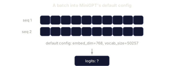
    def __init__(self, vocab_size=50257, embed_dim=768, num_heads=12,
                 num_layers=12, max_seq_len=1024, ff_dim=3072):
        self.embedding = Embedding(vocab_size, embed_dim, max_seq_len)
        self.blocks = [
            TransformerBlock(embed_dim, num_heads, ff_dim)
            for _ in range(num_layers)
        ]
        self.ln_f = LayerNorm(embed_dim)
        self.vocab_size = vocab_size
        self.embed_dim = embed_dim

    def forward(self, token_ids):
        seq_len = token_ids.shape[-1]
        mask = np.triu(np.full((seq_len, seq_len), -1e9), k=1)

        x = self.embedding.forward(token_ids)
        for block in self.blocks:
            x = block.forward(x, mask)
        x = self.ln_f.forward(x)

        logits = x @ self.embedding.token_embed.T
        return logits

    def count_parameters(self):
        total = 0
        total += self.embedding.token_embed.size
        total += self.embedding.pos_embed.size
        for block in self.blocks:
            total += block.attn.W_q.size + block.attn.W_k.size
            total += block.attn.W_v.size + block.attn.W_out.size
            total += block.ffn.W1.size + block.ffn.b1.size
            total += block.ffn.W2.size + block.ffn.b2.size
            total += block.ln1.gamma.size + block.ln1.beta.size
            total += block.ln2.gamma.size + block.ln2.beta.size
        total += self.ln_f.gamma.size + self.ln_f.beta.size
        return total
Look at the weight tying: logits = x @ self.embedding.token_embed.T. The output projection reuses the token embedding matrix, transposed. That saves parameters, but it also means the model uses the same vector space for understanding tokens (embeddings) and predicting them (output).
Step 6: Training Loop
A real 124M-parameter run needs a GPU and PyTorch. This loop shows the mechanics on a small model in pure numpy, with a tiny config (4 layers, 4 heads, 128 dims) to keep it tractable.
def cross_entropy_loss(logits, targets):
    batch, seq_len, vocab_size = logits.shape
    logits_flat = logits.reshape(-1, vocab_size)
    targets_flat = targets.reshape(-1)

    max_logits = logits_flat.max(axis=-1, keepdims=True)
    log_softmax = logits_flat - max_logits - np.log(
        np.exp(logits_flat - max_logits).sum(axis=-1, keepdims=True)
    )

    loss = -log_softmax[np.arange(len(targets_flat)), targets_flat].mean()
    return loss


def train_mini_gpt(text, vocab_size=256, embed_dim=128, num_heads=4,
                   num_layers=4, seq_len=64, num_steps=200, lr=3e-4):
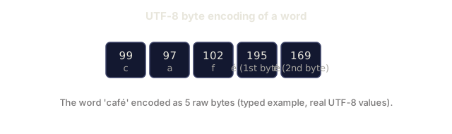
    tokens = np.array(list(text.encode("utf-8")[:2048]))
    model = MiniGPT(
        vocab_size=vocab_size, embed_dim=embed_dim, num_heads=num_heads,
        num_layers=num_layers, max_seq_len=seq_len, ff_dim=embed_dim * 4
    )

    print(f"Model parameters: {model.count_parameters():,}")
    print(f"Training tokens: {len(tokens):,}")
    print(f"Config: {num_layers} layers, {num_heads} heads, {embed_dim} dims")
    print()

    for step in range(num_steps):
        start_idx = np.random.randint(0, max(1, len(tokens) - seq_len - 1))
        batch_tokens = tokens[start_idx:start_idx + seq_len + 1]

        input_ids = batch_tokens[:-1].reshape(1, -1)
        target_ids = batch_tokens[1:].reshape(1, -1)

        logits = model.forward(input_ids)
        loss = cross_entropy_loss(logits, target_ids)

        if step % 20 == 0:
            print(f"Step {step:4d} | Loss: {loss:.4f}")

    return model
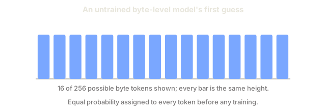
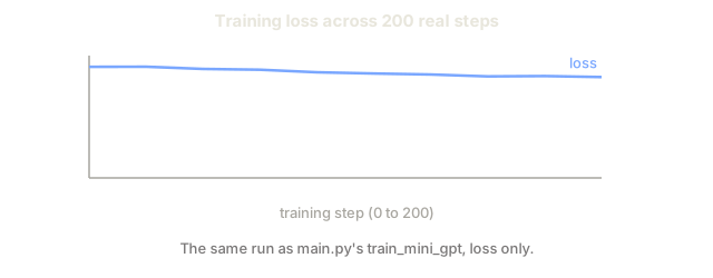
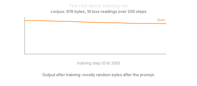
The loss starts near ln(vocab_size), which for a 256-token byte-level vocabulary is ln(256) = 5.55. A random model assigns equal probability to every token. As training progresses the loss drops because the model learns common patterns, like "h" after "t" or a space after a period. In the 200-step demo it only falls from about 5.57 to about 5.05, so it has barely started.
The listing above stops at the loss to keep the focus on the forward pass. The train_mini_gpt in main.py also runs a hand-written backward pass and a plain SGD update (learning rate 3e-4), but only for the FFN weights, the second LayerNorm in each block, the final LayerNorm, and the token embeddings. Attention weights, the first LayerNorm in each block and the position embeddings stay at their random initial values. A production run adds Adam, gradient accumulation, learning rate warmup, and gradient clipping. The forward, loss, backward, update loop stays the same and only the optimizer gets fancier.
Step 7: Text Generation
Generation predicts one token at a time. Each prediction is sampled from the output distribution, or taken greedily as the argmax.
def generate(model, prompt_tokens, max_new_tokens=100, temperature=0.8):
    tokens = list(prompt_tokens)
    seq_len = model.embedding.pos_embed.shape[0]

    for _ in range(max_new_tokens):
        context = np.array(tokens[-seq_len:]).reshape(1, -1)
        logits = model.forward(context)
        next_logits = logits[0, -1, :]

        next_logits = next_logits / temperature
        probs = np.exp(next_logits - next_logits.max())
        probs = probs / probs.sum()

        next_token = np.random.choice(len(probs), p=probs)
        tokens.append(next_token)

    return tokens
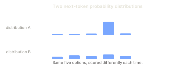
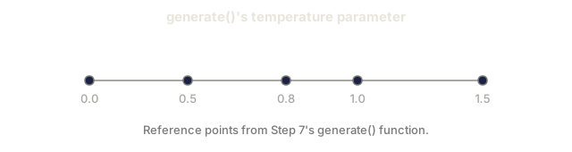
Temperature controls randomness. At 1.0 you sample from the raw distribution. At 0.5 the distribution sharpens and the top choices win more often. At 1.5 it flattens and low-probability tokens get a bigger chance. At 0.0 you get greedy decoding, the highest-probability token.
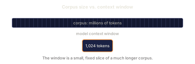
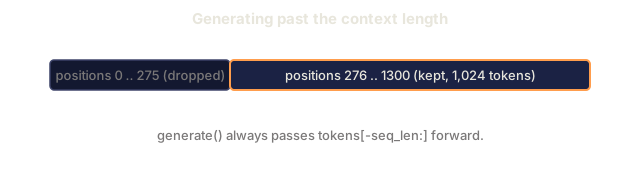
The tokens[-seq_len:] window exists because the model has a maximum context length (1024 for GPT-2), and past that the oldest tokens get dropped. That is the "context window" people talk about.


Use It
Full Training and Generation Demo
corpus = """The transformer architecture has revolutionized natural language processing.
Attention mechanisms allow the model to focus on relevant parts of the input.
Self-attention computes relationships between all pairs of positions in a sequence.
Multi-head attention splits the representation into multiple subspaces.
Each attention head can learn different types of relationships.
The feedforward network provides nonlinear transformations at each position.
Residual connections enable gradient flow through deep networks.
Layer normalization stabilizes training by normalizing activations.
Position embeddings give the model information about token ordering.
The causal mask ensures autoregressive generation during training.
Pre-training on large text corpora teaches the model general language understanding.
Fine-tuning adapts the pre-trained model to specific downstream tasks."""

model = train_mini_gpt(corpus, num_steps=200)

prompt = list("The transformer".encode("utf-8"))
output_tokens = generate(model, prompt, max_new_tokens=100, temperature=0.8)
generated_text = bytes(output_tokens).decode("utf-8", errors="replace")
print(f"\nGenerated: {generated_text}")
Expect noise, not prose. The corpus is about 880 bytes, the run is 200 steps, and the update is partial SGD, so the loss only slips from about 5.57 to about 5.05 and the generated text is mostly random bytes after the prompt. GPT-2 gets its quality from 40GB of training data and the full 124M-parameter architecture. Output quality isn't the point. You can trace each step: embedding lookup, attention, feedforward, logit projection, softmax, sampling.
Ship It
This lesson produces outputs/prompt-gpt-architecture-analyzer.md, a prompt that analyzes the architecture choices in a GPT-style model. Feed it a model card or technical report and it breaks down the parameter allocation, attention design, and scaling decisions.
I'd run main.py before rereading the architecture. It prints a parameter breakdown and a memory estimate, then trains the small 4-layer, 128-dim config on a short corpus and generates from a prompt. Its GPT-2 Small row comes out at 124,402,944, not the 124,438,272 in the table, so it's worth working out where the gap comes from instead of trusting either number.
Read the training loop with one thing in mind: the backward pass in main.py is hand-written, and it only reaches the feedforward weights, the second layer norm in each block, the final layer norm, and the token embedding. The attention weights, the first layer norm in each block, and the position embeddings stay where they started, and the update is plain SGD, not Adam. So the printed loss is a real next-token loss, but a falling curve doesn't show that attention has learned anything. Exercise 5 is a good place to see how far that gets you.
My bet is that weight tying is the line worth rereading until it feels boring. logits = x @ self.embedding.token_embed.T reuses the embedding matrix as the output head, which is where the 38M saving comes from. Once you see that, the parameter table stops looking like a list of numbers to memorize.
I'd also keep the ReLU in proportion. It stands in for GELU here, and I'd swap it back as soon as you want numbers that compare with GPT-2. That is exercise 2.
Exercises
-
Modify the model to use 24 layers and 16 heads instead of 12/12. Count the parameters. How does doubling the depth compare to doubling the width (embedding dimension)?
-
Implement the GELU activation function (GELU(x) = x * 0.5 * (1 + erf(x / sqrt(2)))) and replace the ReLU in the feedforward network. Run training for 500 steps with each activation and compare the final loss.
-
Add a KV cache to the generation function. Store K and V tensors for each layer after the first forward pass, and reuse them for subsequent tokens. Measure the speedup: generate 200 tokens with and without the cache and compare wall-clock time.
-
Implement top-k sampling (only consider the k highest-probability tokens) and top-p sampling (nucleus sampling: consider the smallest set of tokens whose cumulative probability exceeds p). Compare the output quality at temperature 0.8 with top-k=50 vs top-p=0.95.
-
Build a training loss curve plotter. Train the model for 1000 steps and plot loss vs step. Identify the three phases: rapid initial descent (learning common bytes), slower middle phase (learning byte patterns), and plateau (overfitting on the small corpus). The shape of this curve is the same whether you are training a 128-dim model or GPT-4.
Key Terms
| Term | What people say | What it actually means |
|---|---|---|
| Autoregressive | "It generates one word at a time" | Each output token is conditioned on all previous tokens so the model predicts P(token_n | token_0, ..., token_{n-1}) |
| Causal mask | "It can't see the future" | An upper-triangular matrix of -infinity values that prevents attention to future positions during training |
| Multi-head attention | "Multiple attention patterns" | Splitting Q, K, V into parallel heads (e.g., 12 heads of 64 dims each for GPT-2) so each head can learn different relationship types |
| KV Cache | "Caching for speed" | Storing computed Key and Value tensors from previous tokens to avoid redundant computation during autoregressive generation |
| Prefill | "Processing the prompt" | The first inference phase where all prompt tokens are processed in parallel, compute-bound on GPU FLOPS |
| Decode | "Generating tokens" | The second inference phase where tokens are generated one at a time, memory-bound on GPU bandwidth |
| Weight tying | "Sharing embeddings" | Using the same matrix for input token embeddings and the output projection head, which saves 38M params in GPT-2 |
| Residual connection | "Skip connection" | Adding the input directly to the output of a sublayer (x + sublayer(x)), which enables gradient flow in deep networks |
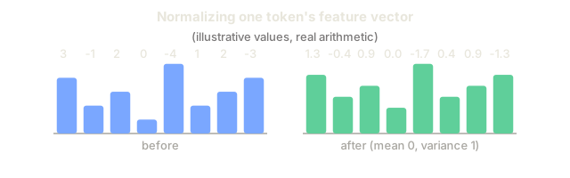
| Layer normalization | "Normalizing activations" | Normalizing across the feature dimension to mean 0 and variance 1, with learnable scale and bias parameters |
| Cross-entropy loss | "How wrong the predictions are" | -log(probability assigned to the correct next token), averaged over all positions. The standard LLM training objective |
Further Reading
- Radford et al., 2019: "Language Models are Unsupervised Multitask Learners" (GPT-2): the GPT-2 paper that introduced the 124M to 1.5B parameter family
- Vaswani et al., 2017: "Attention Is All You Need": the original transformer paper with scaled dot-product attention and multi-head attention
- Llama 3 Technical Report: how Meta scaled the GPT architecture to 405B parameters with 16K GPUs
- Pope et al., 2022: "Efficiently Scaling Transformer Inference": the paper that formalized prefill vs decode and KV cache analysis