Monte Carlo Methods — Learning from Complete Episodes
Dynamic programming needs a model. Monte Carlo needs nothing but episodes: run the policy, watch the returns, average them. It's the simplest idea in RL, and the one that unlocks everything downstream.
Learning Objectives
- Explain why Monte Carlo methods only need the ability to sample from an environment, not a known transition model, and state the variance-for-applicability tradeoff versus dynamic programming.
- Distinguish first-visit from every-visit Monte Carlo, derive the incremental mean update, and explain how swapping in a constant step size α turns the sample-average estimator into the bridge from MC to TD.
- Implement first-visit MC policy evaluation and ε-greedy MC control from raw episode rollouts in code, and validate the result against Lesson 02's dynamic-programming baseline.
- Explain why exploration becomes a problem under MC but not DP, and describe the three fixes, exploring starts, ε-greedy, and off-policy importance sampling, including why importance-sampling variance grows with episode horizon.
The Problem
Dynamic programming is elegant, but it assumes you can query P(s' | s, a) for every state and action. Almost nothing in the real world offers that. A robot can't analytically compute the distribution over camera pixels after a joint torque. A pricing algorithm can't integrate over every possible customer reaction. An LLM can't enumerate every possible continuation after a token.
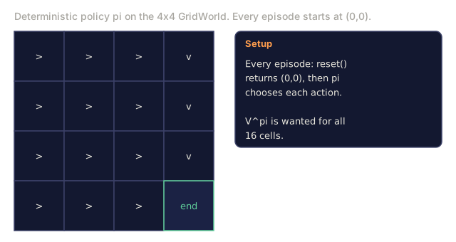
What you need instead is a method that only requires the ability to sample from the environment: run the policy, collect a trajectory s_0, a_0, r_1, s_1, a_1, r_2, …, s_T, and use it to estimate values. That's Monte Carlo.
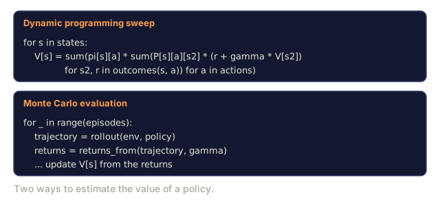
The shift from DP to MC matters philosophically: you trade a known model with exact backups for sampled rollouts averaged into a return. Variance goes up, but applicability explodes. Every RL algorithm after this lesson (TD, Q-learning, REINFORCE, PPO, GRPO) is a Monte Carlo estimator at heart, sometimes with bootstrapping layered on top.
The Concept

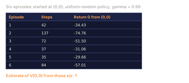
The core idea, in one line: V^π(s) = E_π[G_t | s_t = s] ≈ (1/N) Σ_i G^{(i)}(s) where G^{(i)}(s) are observed returns following visits to s under policy π.
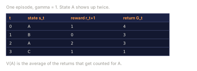
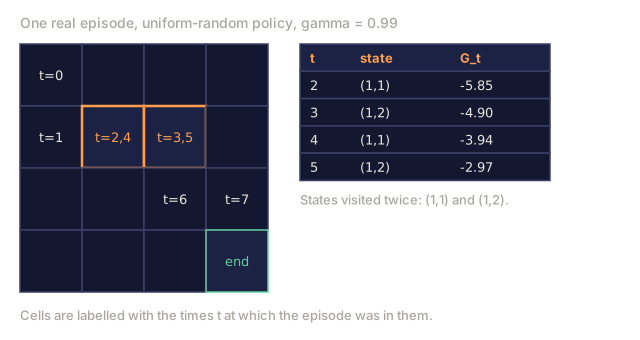
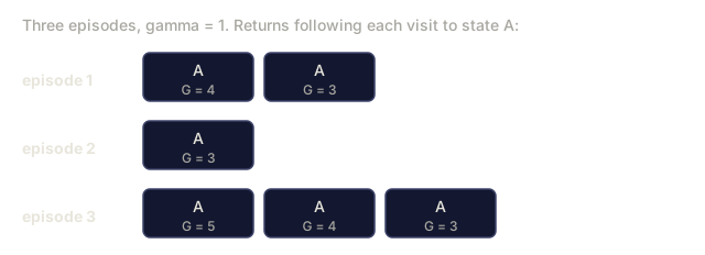
First-visit vs every-visit MC. Given an episode that visits state s multiple times, first-visit MC counts only the return from the first visit; every-visit MC counts all of them. Both are unbiased in the limit. First-visit is easier to analyze, since the samples are iid. Every-visit uses more data per episode and typically converges faster in practice.
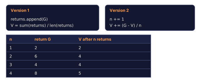
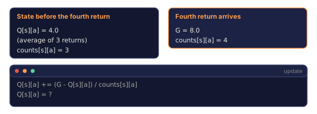
Incremental mean. Instead of storing all returns, update the running average:
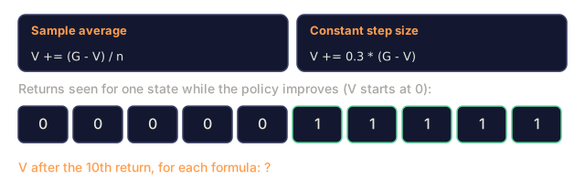
V_n(s) = V_{n-1}(s) + (1/n) [G_n - V_{n-1}(s)]
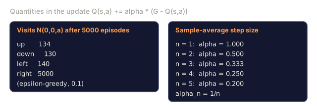
Reorganize that into V_new = V_old + α · (target - V_old) with α = 1/n. Swap the 1/n for a constant step-size α ∈ (0, 1) and you get a non-stationary MC estimator that tracks a moving π. That single substitution is the entire jump from MC to TD, and from there to every modern RL algorithm.
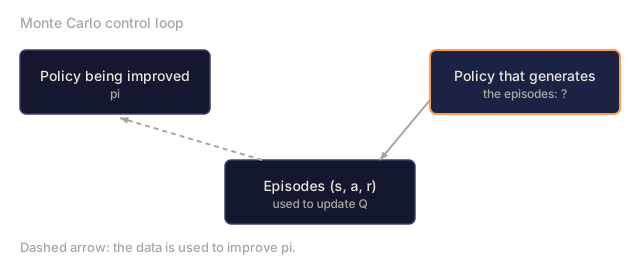
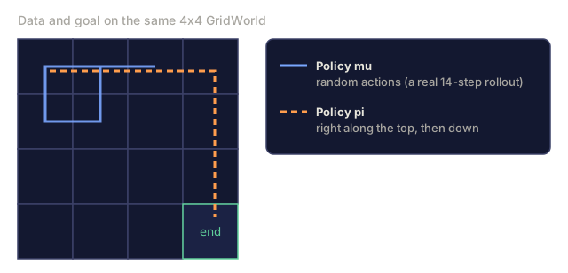
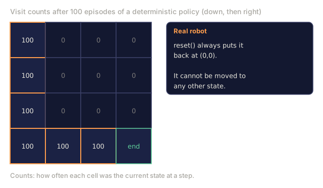
Exploration is now a problem. DP touched every state by enumeration; MC only sees states the policy actually visits. If π is deterministic, whole regions of the state space never get sampled, and their value estimates sit at zero forever. Three fixes, in historical order:
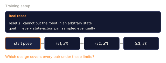
- Exploring starts. Start each episode from a random (s, a) pair. This guarantees coverage, but it's unrealistic in practice: you can't reset a robot into an arbitrary state.
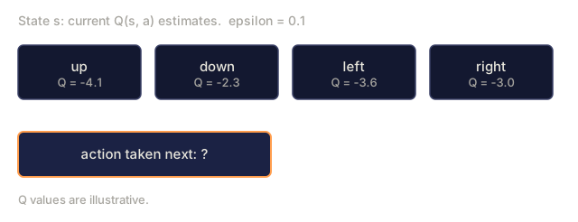
- ε-greedy. Act greedy with respect to the current Q, but with probability
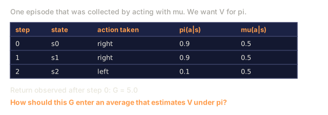
εpick a random action instead. All state-action pairs get sampled asymptotically. - Off-policy MC. The first two fixes are on-policy: the same policy you're improving is the one generating the data. Off-policy MC drops that constraint. Collect data under a behavior policy
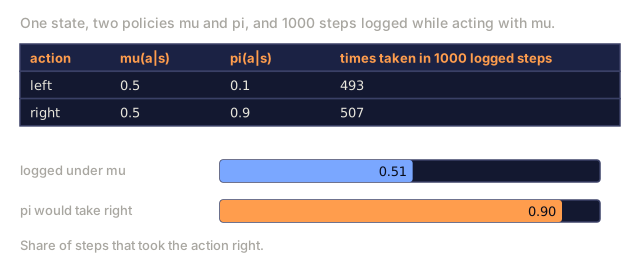
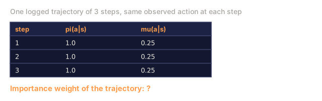
μ, then learn about a different target policyπby reweighting each observed return by the probability ratioπ(a|s)/μ(a|s), a correction called importance sampling. Variance is high, but this is the bridge to replay-buffer methods like DQN.
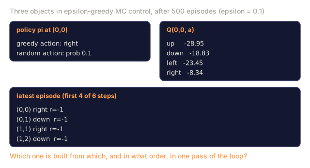
Monte Carlo Control. Evaluate → improve → evaluate, the same loop as policy iteration, except evaluation is now sampling-based:
- Run
π, get an episode. - Update
Q(s, a)from the observed returns. - Make
πε-greedy with respect toQ. - Repeat.
It converges to Q* and π* with probability 1 under mild conditions: every pair visited infinitely often, and α satisfying Robbins-Monro.
Build It
Step 1: rollout → list of (s, a, r)
def rollout(env, policy, max_steps=200):
    trajectory = []
    s = env.reset()
    for _ in range(max_steps):
        a = policy(s)
        s_next, r, done = env.step(s, a)
        trajectory.append((s, a, r))
        s = s_next
        if done:
            break
    return trajectory
No model, only env.reset() and env.step(s, a). Same interface as a gym environment but stripped down.
Step 2: compute returns (reverse sweep)
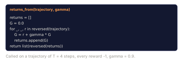
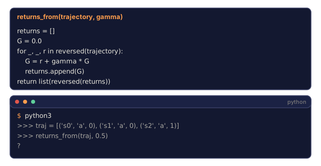
def returns_from(trajectory, gamma):
    returns = []
    G = 0.0
    for _, _, r in reversed(trajectory):
        G = r + gamma * G
        returns.append(G)
    return list(reversed(returns))
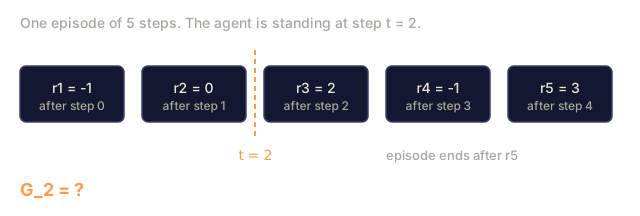
One pass, O(T). The backward recurrence G_t = r_{t+1} + γ G_{t+1} avoids re-summing.
Step 3: first-visit MC evaluation
def mc_policy_evaluation(env, policy, episodes, gamma=0.99):
    V = defaultdict(float)
    counts = defaultdict(int)
    for _ in range(episodes):
        trajectory = rollout(env, policy)
        returns = returns_from(trajectory, gamma)
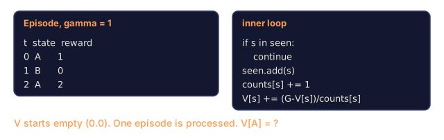
        seen = set()
        for t, ((s, _, _), G) in enumerate(zip(trajectory, returns)):
            if s in seen:
                continue
            seen.add(s)
            counts[s] += 1
            V[s] += (G - V[s]) / counts[s]
    return V
Three lines do the work: mark state as seen on first visit, increment count, update running mean.
Step 4: ε-greedy MC control (on-policy)
def mc_control(env, episodes, gamma=0.99, epsilon=0.1):
    Q = defaultdict(lambda: {a: 0.0 for a in ACTIONS})
    counts = defaultdict(lambda: {a: 0 for a in ACTIONS})

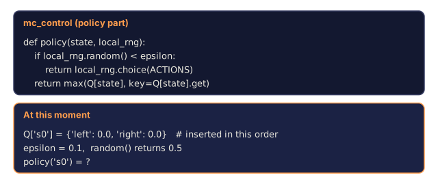
    def policy(s):
        if random() < epsilon:
            return choice(ACTIONS)
        return max(Q[s], key=Q[s].get)

    for _ in range(episodes):
        trajectory = rollout(env, policy)
        returns = returns_from(trajectory, gamma)
        seen = set()
        for (s, a, _), G in zip(trajectory, returns):
            if (s, a) in seen:
                continue
            seen.add((s, a))
            counts[s][a] += 1
            Q[s][a] += (G - Q[s][a]) / counts[s][a]
    return Q, policy
Step 5: compare to DP gold standard
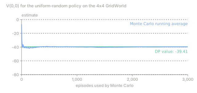
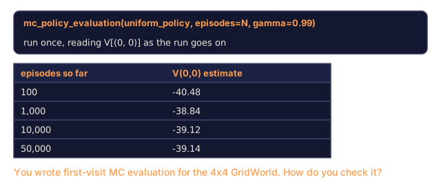
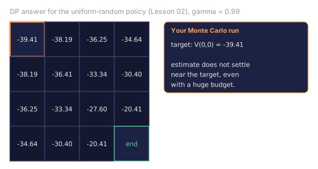
Your MC estimate of V^π should agree with the DP result from Lesson 02 as episodes → ∞. In practice, 50,000 episodes on 4×4 GridWorld gets you within ~0.1 of the DP answer.
Pitfalls
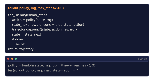
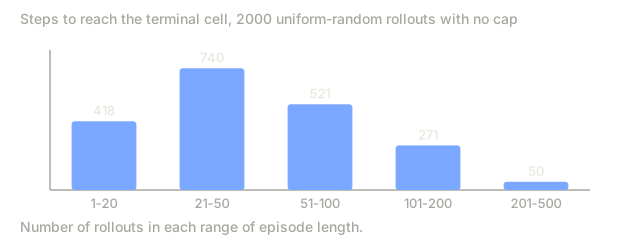
- Infinite episodes. MC requires episodes to terminate. If your policy can loop forever, cap
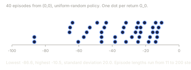
max_stepsand treat hitting that cap as an implicit failure. GridWorld with a random policy routinely times out, and that's normal as long as you count it correctly. - Variance. MC uses full returns, so on long episodes the variance is huge: one unlucky reward at the end shifts
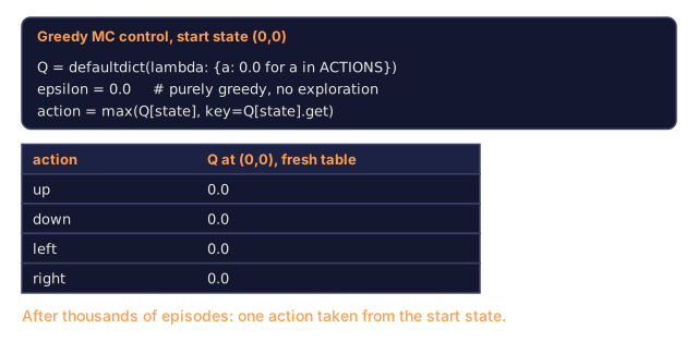
V(s_0)by the same amount. TD methods (Lesson 04) cut this down by bootstrapping. - State coverage. Greedy MC on a fresh Q with ties will only ever try one action. You have to explore, whether through ε-greedy, exploring starts, or UCB.
- Non-stationary policies. If
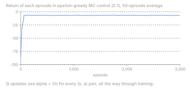
πchanges, as it does in MC control, old returns come from a different policy. Constant-α MC handles that; sample-average MC does not. - Off-policy importance sampling. The weights
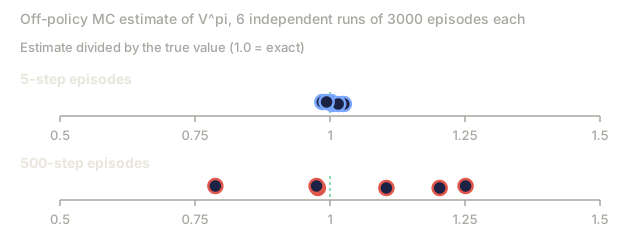
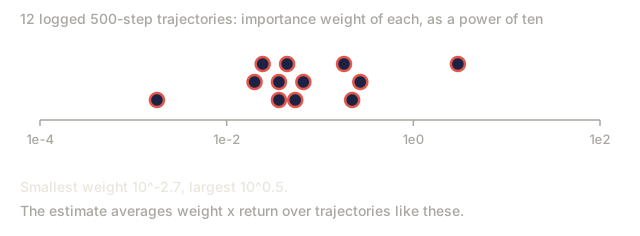
π(a|s)/μ(a|s)multiply across a trajectory, so variance explodes with horizon. Per-decision IS reweights each reward individually instead of the whole return, and weighted IS normalizes by the sum of weights instead of the episode count; both cut variance relative to plain IS. Cap it with one of those, or switch to TD.
Use It
The 2026 role of Monte Carlo methods:
| Use case | Why MC |
|---|---|
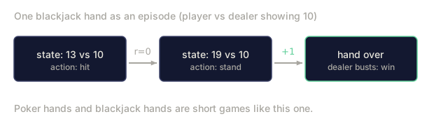
| Short-horizon games (blackjack, poker) | Episodes terminate naturally; returns are clean. |
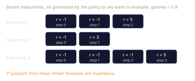
| Offline evaluation of a logged policy | Average discounted returns over stored trajectories. |
| Monte Carlo Tree Search (AlphaZero) | MC rollouts from tree leaves guide selection. |
| LLM RL evaluation | Compute average reward over sampled completions for a given policy. |
| Baseline estimation in PPO | The advantage target A_t = G_t - V(s_t) uses an MC G_t. |
| Teaching RL | Simplest algorithm that actually works: strip out bootstrapping and you see the core. |
Modern deep-RL algorithms (PPO, SAC) interpolate between pure MC (full returns) and pure TD (one-step bootstrap) via n-step returns or GAE. Both endpoints are instances of the same estimator.
Ship It
Save as outputs/skill-mc-evaluator.md:
---
name: mc-evaluator
description: Evaluate a policy via Monte Carlo rollouts and produce a convergence report with DP-comparison if available.
version: 1.0.0
phase: 9
lesson: 3
tags: [rl, monte-carlo, evaluation]
---

Given an environment (episodic, with reset+step API) and a policy, output:

1. Method. First-visit vs every-visit MC. Reason.
2. Episode budget. Target number, variance diagnostic, expected standard error.
3. Exploration plan. ε schedule (if needed) or exploring starts.
4. Gold-standard comparison. DP-optimal V* if tabular; otherwise a bound from a Q-learning / PPO baseline.
5. Termination check. Max-step cap, timeouts, handling of non-terminating trajectories.

Refuse to run MC on non-episodic tasks without a finite horizon cap. Refuse to report V^π estimates from fewer than 100 episodes per state for tabular tasks. Flag any policy with zero-variance actions as an exploration risk.The first time this clicked for me wasn't the math, it was watching the numbers converge. Run a few thousand episodes of the random policy against the DP answer from Lesson 02, and V(0,0) crawls toward the exact value: noisy at first, then unmistakably heading somewhere specific. That's the moment Monte Carlo stops being an abstract idea about sampling and turns into something you can watch happen in real time. If your estimate refuses to settle, don't reach for a bigger episode budget first. Check that your policy actually reaches every state you're trying to evaluate. Most 'MC isn't converging' bugs I've run into turn out to be exploration bugs wearing a variance costume.
Exercises
- Easy. Implement first-visit MC evaluation of the uniform-random policy on 4×4 GridWorld. Run 10,000 episodes. Plot
V(0,0)as a function of episode count against the DP answer. - Medium. Implement ε-greedy MC control with
ε ∈ {0.01, 0.1, 0.3}. Compare mean return after 20,000 episodes. What does the curve look like? Where does the bias-variance tradeoff live? - Hard. Implement off-policy MC with importance sampling: collect data under uniform-random policy
μ, estimateV^πfor the deterministic optimal policyπ. Compare plain IS vs per-decision IS vs weighted IS. Which has lowest variance?
Key Terms
| Term | What people say | What it actually means |
|---|---|---|
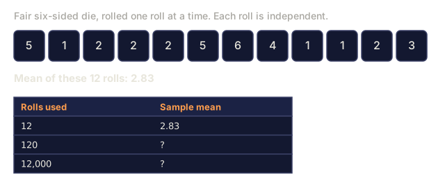
| Monte Carlo | "Random sampling" | Estimate expectations by averaging over iid samples from the distribution. |
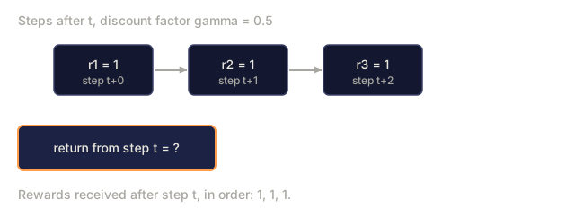
Return G_t | "Future reward" | Sum of discounted rewards from step t to episode end: Σ_{k≥0} γ^k r_{t+k+1}. |
| First-visit MC | "Count each state once" | Only the first visit in an episode contributes to the value estimate. |
| Every-visit MC | "Use all visits" | Every visit contributes; slightly biased but more sample-efficient. |
| ε-greedy | "Exploration noise" | Pick greedy action with prob 1-ε; random action with prob ε. |
| Importance sampling | "Correcting for sampling from the wrong distribution" | Reweight returns by π(a|s)/μ(a|s) products to estimate V^π from μ data. |
| On-policy | "Learn from my own data" | Target policy = behavior policy. Vanilla MC, PPO, SARSA. |
| Off-policy | "Learn from someone else's data" | Target policy ≠ behavior policy. Importance-sampled MC, Q-learning, DQN. |
Further Reading
- Sutton & Barto (2018). Ch. 5 — Monte Carlo Methods: the canonical treatment.
- Singh & Sutton (1996). Reinforcement Learning with Replacing Eligibility Traces: first-visit vs every-visit analysis.
- Precup, Sutton, Singh (2000). Eligibility Traces for Off-Policy Policy Evaluation: off-policy MC and variance control.
- Mahmood et al. (2014). Weighted Importance Sampling for Off-Policy Learning: modern low-variance IS estimators.
- Tesauro (1995). TD-Gammon, A Self-Teaching Backgammon Program: the first large-scale empirical demonstration of MC/TD self-play converging to superhuman play, and the conceptual precursor to every lesson in the second half of this phase.
Code
- main.py (python, 143 lines)