TAI BUI
Back to curriculum
BuildPython

Dynamic Programming — Policy Iteration & Value Iteration

Dynamic programming is RL with cheating. You already know the transition and reward functions; you just iterate the Bellman equation until `V` or `π` stops moving. It is the benchmark every sampling-based method tries to approach.

TIME: ~75 minutesPREREQUISITES: Phase 9 · 01 (MDPs)

Learning Objectives

  • Distinguish policy iteration from value iteration as two ways of fixed-point-iterating the Bellman equation, and implement both for a tabular MDP.
  • Explain why the Bellman operator's gamma-contraction property guarantees convergence to a unique fixed point, and state what breaks when gamma is not less than 1.
  • Diagnose the recurring dynamic-programming bugs (unguarded terminal states, sup-norm vs. average convergence checks, unstable tie-breaking, state-space blowup) before they cause silent failures.
  • Connect policy iteration and value iteration to Generalized Policy Iteration (GPI), and explain why Q-learning, actor-critic, and PPO are all instances of the same loop.

The Problem

You have an MDP with a known model: you can query P(s' | s, a) and R(s, a, s') for any state-action pair. An inventory manager knows the demand distribution. A board game has deterministic transitions. A gridworld is four lines of Python. You have a model.

Model-free RL (Q-learning, PPO, REINFORCE) was built for the opposite case: no model, only samples from the environment. When you do have a model, dynamic programming gets you there faster and exactly. Bellman designed these methods in 1957, and they still define correctness. When people say "optimal policy for this MDP," they mean the policy DP would return.

You need them in 2026 for three reasons. First, every tabular environment in RL research (GridWorld, FrozenLake, CliffWalking) is solved with DP to produce the gold-standard policy. Second, exact values let you debug sampling methods: if Q-learning's estimate for V*(s_0) disagrees with the DP answer by 30%, your Q-learning has a bug. Third, modern offline RL and planning methods (MCTS, AlphaZero's search, model-based RL in Phase 9 · 10) all iterate a Bellman backup over a learned or given model.
Warm-up0/3
1. In reinforcement learning, what is a policy?Warm-up
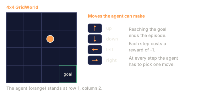
A 4x4 grid with a goal cell at the bottom right and the agent at row 1, column 2, beside the four available moves (up, down, left, right) and notes that each step costs -1 and reaching the goal ends the episode.
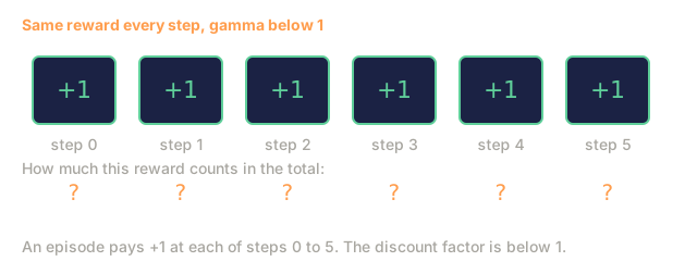
2. In an MDP, what does a discount factor gamma below 1 do to future rewards?Warm-up
Six boxes for steps 0 to 5, each paying a reward of +1, with a question mark under each for how much that reward counts in the total, and a note that the discount factor is below 1.
3. An agent is told, for every state and action, the exact probability of each next state and the reward that follows. What is this knowledge called?Warm-up
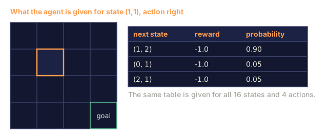
A 4x4 grid with state (1,1) outlined beside a table for action right in that state: next state (1,2) with reward -1.0 and probability 0.90, next state (0,1) with -1.0 and 0.05, next state (2,1) with -1.0 and 0.05, and a note that such a table exists for every state and action.
Values from the lesson's transitions function with slip 0.1.
Check: The Problem0/3
1. Why can dynamic programming solve an MDP exactly, while model-free methods like Q-learning must estimate from samples?Explain
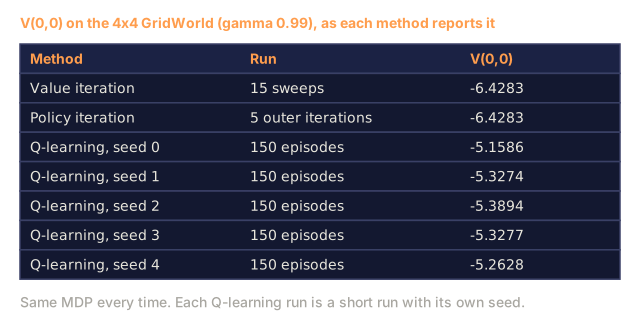
A table of the value of the start cell on the 4x4 GridWorld: value iteration and policy iteration both give -6.4283 and five short Q-learning runs with seeds 0 to 4 give different values.
Computed here: value and policy iteration from the lesson's code; Q-learning alpha 0.1, epsilon 0.1, 150 episodes per seed.
2. Although model-free methods dominate practice, what does dynamic programming still define for a tabular MDP?Explain
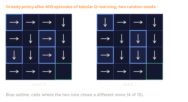
Two 4x4 grids of arrows, the greedy moves after 400 episodes of tabular Q-learning with seed 0 and seed 1, with the 4 cells where the two runs differ outlined in blue.
Computed here: alpha 0.1, epsilon 0.1, gamma 0.99, lesson GridWorld with slip 0.1.
3. Why do exact DP values help you debug a sampling-based method such as Q-learning?Explain
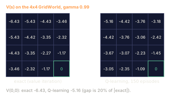
Two 4x4 value grids on the GridWorld: the exact values from value iteration and the values from a 150-episode tabular Q-learning run, with V(0,0) printed for both (-6.43 and -5.16).
Computed here: one short Q-learning run (150 episodes, seed 0, alpha 0.1, epsilon 0.1), not the lesson's own result.

The Concept

Policy iteration and value iteration, side by side

Two algorithms, both fixed-point iteration on Bellman.

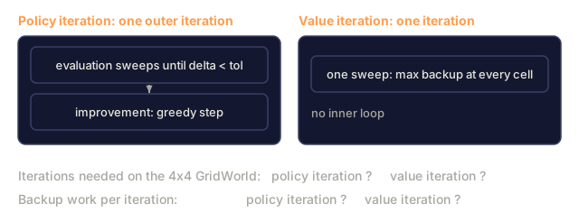
Policy iteration. Alternates two steps until the policy stops changing.

  1. Evaluation: given policy π, compute V^π by repeatedly applying V(s) ← Σ_a π(a|s) Σ_{s',r} P(s',r|s,a) [r + γ V(s')] until it converges.
  2. Improvement: given V^π, make π greedy w.r.t. V^π: π(s) ← argmax_a Σ_{s',r} P(s',r|s,a) [r + γ V(s')].

Convergence is guaranteed because (a) each improvement step either keeps π the same or strictly increases V^π for some state, and (b) the space of deterministic policies is finite. Usually converges in ~5–20 outer iterations, even for large state spaces.

Value iteration. Collapses evaluation and improvement into one sweep. Apply the Bellman optimality equation:

V(s) ← max_a Σ_{s',r} P(s',r|s,a) [r + γ V(s')]

Repeat until max_s |V_{new}(s) - V(s)| < ε, then extract the policy at the end by taking the greedy action. It's strictly faster per iteration (no inner evaluation loop), but it typically needs more iterations to converge.

Generalized policy iteration (GPI). The unifying framing. Value function and policy are locked in a two-way improvement loop, and any method that drives both toward mutual consistency — async value iteration, modified policy iteration, Q-learning, actor-critic, PPO — is an instance of GPI.

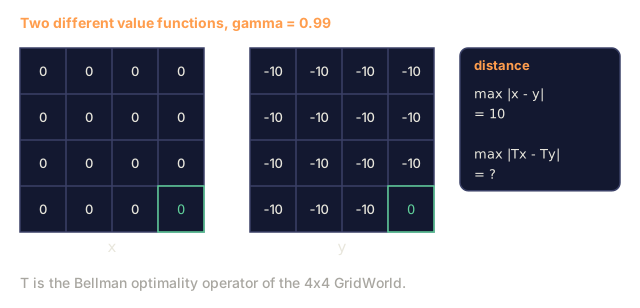
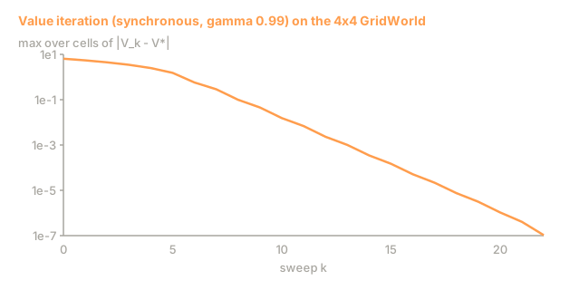
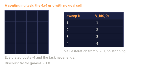
Why γ < 1 matters. The Bellman operator is a γ-contraction in the sup-norm: ||T V - T V'||_∞ ≤ γ ||V - V'||_∞. Contraction implies a unique fixed point and geometric convergence. Drop γ < 1 and you lose the guarantee: you need a finite horizon or an absorbing terminal state.
Check: The Concept0/13
1. What is policy iteration?Define
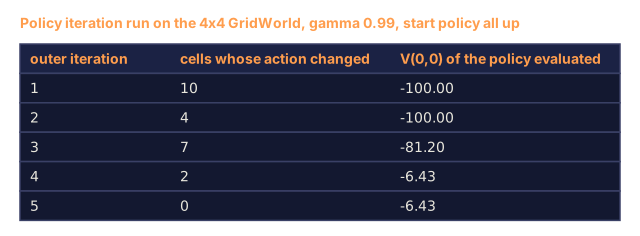
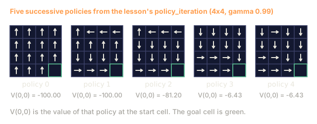
Five 4x4 grids of arrows, policy 0 to policy 4, each with its value at the start cell: -100.00, -100.00, -81.20, -6.43 and -6.43.
Computed with the lesson's GridWorld code. Policy 0 is all up.
2. What is value iteration, and how does it differ from policy iteration?Define
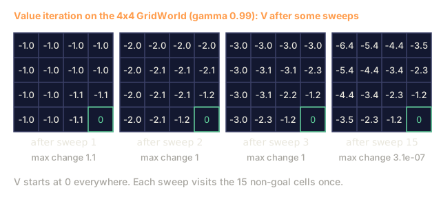
Four 4x4 value grids from value iteration on the GridWorld at gamma 0.99, after sweeps 1, 2, 3 and 15, with the largest change in each sweep printed below (1.1, 1, 1 and 3.1e-07).
Computed with the lesson's value iteration, in place, starting from V = 0.
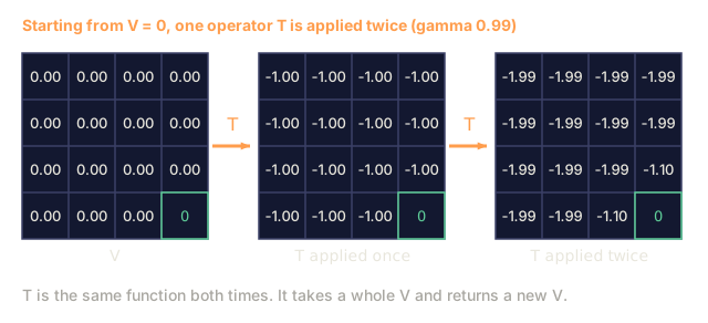
3. What is the Bellman operator T used by value iteration?Define
Three 4x4 value grids joined by arrows labelled T: V equal to 0 everywhere, then the grid after one application (-1.00 in every cell except 0 at the goal), then the grid after a second application, with values from -1.99 to -1.00 near the goal.
Computed with the lesson's GridWorld model, synchronous, goal pinned at 0.
4. What does it mean for an operator T to be a contraction with factor gamma below 1?Define
Two 4x4 value grids x (all 0) and y (-10 in every cell except 0 at the goal) with the sup-norm distance between them equal to 10, and a card asking for the distance after applying T to each, left as a question mark.
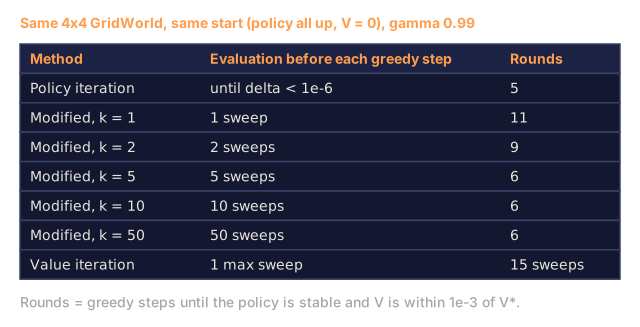
5. What is Generalized Policy Iteration (GPI)?Define
A table of runs on the 4x4 GridWorld listing how much evaluation each method does before each greedy step (until delta below 1e-6 for policy iteration, k sweeps for modified policy iteration with k from 1 to 50, one max sweep for value iteration) and the number of rounds each needed.
Computed here. Value iteration counts sweeps, its policy is read off at the end.
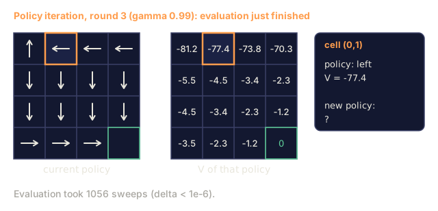
6. In policy iteration, what does the improvement step do?Explain
Two 4x4 grids for round 3 of policy iteration: the current policy as arrows and the value of that policy in each cell (from -81.2 at the top left to 0 at the goal), with cell (0,1) outlined (policy left, V -77.4), and a card asking for its new policy.
Computed with the lesson's code. Goal cell is green.
7. Why is policy iteration guaranteed to terminate?Explain
A table of the five outer iterations of policy iteration on the 4x4 GridWorld listing the number of cells whose action changed (10, 4, 7, 2, 0) and V(0,0) of the evaluated policy (-100.00, -100.00, -81.20, -6.43, -6.43).
Computed with the lesson's code.
8. Value iteration has no inner evaluation loop. What trade-off does that create against policy iteration?Explain
Two panels: one policy iteration step drawn as a box of evaluation sweeps until delta is below tol followed by a greedy improvement box, and one value iteration step drawn as a single sweep of max backups with no inner loop, with the iteration counts and the work per iteration for each left as question marks.
9. Why does the contraction property of the Bellman operator guarantee that value iteration converges?Explain
A log-scale plot of the largest distance between the value function after k sweeps of value iteration and V*, for k from 0 to 21, starting at 6.43 and falling to about 4e-07 by sweep 21.
Computed with the lesson's model; V* from converged value iteration.
10. On an infinite-horizon task, what is lost when gamma is not below 1, and what can restore a guarantee?Explain
A 4x4 grid with no goal cell, a note that every step costs -1, the task never ends and gamma is 1.0, and a table of V(0,0) in value iteration sweeps 1 to 4 equal to -1, -2, -3 and -4.
Computed here with the lesson's slip model and no absorbing cell.
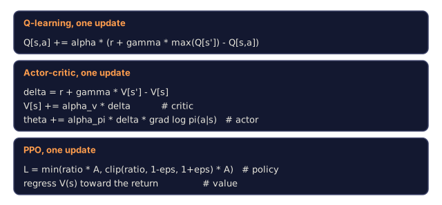
11. Why can the lesson call Q-learning, actor-critic and PPO instances of GPI?Explain
Three code cards with one update of each method: the Q-learning rule on Q[s,a], the actor-critic critic and actor updates, and the PPO clipped objective with a value regression line.
Standard textbook forms, typed here.
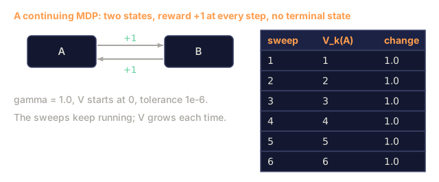
12. You set gamma = 1.0 on an infinite-horizon MDP with no terminal state, and V keeps growing every sweep instead of settling. Which guarantee did you lose?Analyze
Two states A and B joined by arrows that each pay +1, with no terminal state, and a table of value iteration at gamma 1.0 where V(A) is 1, 2, 3, 4, 5, 6 after sweeps 1 to 6 and the change each sweep is 1.0.
Computed here. Typed MDP, not from the lesson's GridWorld.
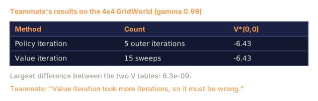
13. A teammate says value iteration must be wrong, because it took far more iterations than policy iteration yet gives the same V*. Are they right?Analyze
A table of results on the 4x4 GridWorld: policy iteration took 5 outer iterations and value iteration 15 sweeps, both giving V*(0,0) = -6.43, with the largest difference between the two tables 6.3e-09 and the teammate's complaint quoted.

Build It

Step 1: build the GridWorld MDP model

Use the same 4×4 GridWorld from Lesson 01. We add a stochastic variant: with probability 0.1 the agent slips to a random perpendicular direction.

python
SLIP = 0.1
 
def transitions(state, action):
    if state == TERMINAL:
        return [(state, 0.0, 1.0)]
    outcomes = []
    for direction, prob in action_probs(action):
        outcomes.append((apply_move(state, direction), -1.0, prob))
    return outcomes

transitions(s, a) returns a list of (s', r, p). This is the entire model.

Step 2: policy evaluation

Given a policy π(s) = {action: prob}, iterate the Bellman equation until V stops moving:

python
def policy_evaluation(policy, gamma=0.99, tol=1e-6):
    V = {s: 0.0 for s in states()}
    while True:
        delta = 0.0
        for s in states():
            v = sum(pi_a * sum(p * (r + gamma * V[s_prime])
                              for s_prime, r, p in transitions(s, a))
                   for a, pi_a in policy(s).items())
            delta = max(delta, abs(v - V[s]))
            V[s] = v
        if delta < tol:
            return V

Step 3: policy improvement

Replace π with the greedy policy w.r.t. V. If π did not change, return: you're already at the optimum.

python
def policy_improvement(V, gamma=0.99):
    new_policy = {}
    for s in states():
        best_a = max(
            ACTIONS,
            key=lambda a: sum(p * (r + gamma * V[s_prime])
                              for s_prime, r, p in transitions(s, a)),
        )
        new_policy[s] = best_a
    return new_policy

Step 4: stitch them together

python
def policy_iteration(gamma=0.99):
    policy = {s: "up" for s in states()}   # arbitrary start
    for _ in range(100):
        V = policy_evaluation(lambda s: {policy[s]: 1.0}, gamma)
        new_policy = policy_improvement(V, gamma)
        if new_policy == policy:
            return V, policy
        policy = new_policy

Typical convergence on 4×4: 4–6 outer iterations. Outputs V*(0,0) ≈ -6 and a policy that strictly decreases the step count.

Step 5: value iteration (the one-loop version)

python
def value_iteration(gamma=0.99, tol=1e-6):
    V = {s: 0.0 for s in states()}
    while True:
        delta = 0.0
        for s in states():
            v = max(sum(p * (r + gamma * V[s_prime])
                       for s_prime, r, p in transitions(s, a))
                   for a in ACTIONS)
            delta = max(delta, abs(v - V[s]))
            V[s] = v
        if delta < tol:
            break
    policy = policy_improvement(V, gamma)
    return V, policy

Same fixed point, fewer lines of code.
Check: Build It0/7
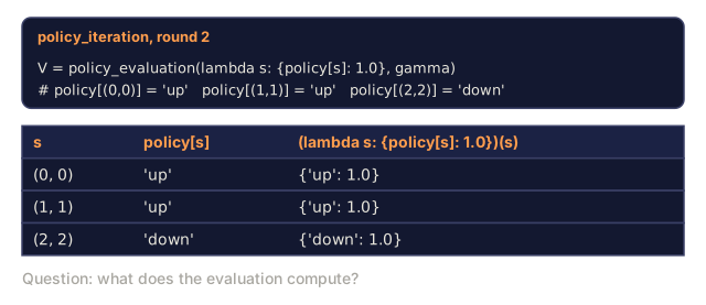
1. In policy_iteration, policy_evaluation(lambda s: {policy[s]: 1.0}, gamma) is called. What does it compute?Apply
The policy_evaluation call with the lambda {policy[s]: 1.0} inside policy_iteration, and a table showing what the lambda returns for cells (0,0), (1,1) and (2,2) of the current policy, each a one-entry dictionary with probability 1.0.
Policy shown is the one after the first improvement, from the lesson's code.
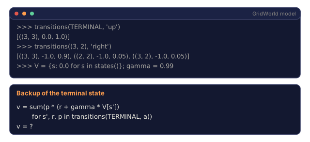
2. With V starting at 0, transitions(TERMINAL, a) returns [(TERMINAL, 0.0, 1.0)]. What does a Bellman backup of the terminal state compute?Apply
A Python session printing transitions(TERMINAL, 'up') as a single self-loop with reward 0.0 and probability 1.0 and transitions((3, 2), 'right') for a normal cell, with all values in V at 0.0 and gamma 0.99, above the backup formula applied to the terminal state with its result left as a question mark.
Output from the lesson's transitions function.
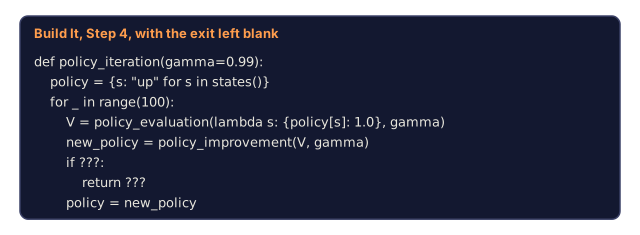
3. In policy_iteration, when does the loop return, and what does it return?Apply
The lesson's policy_iteration function with its exit condition and returned values blanked: it starts from an all-up policy, loops up to 100 times evaluating the policy and computing new_policy with policy_improvement, has an if with question marks followed by a return with question marks, and otherwise sets policy to new_policy.
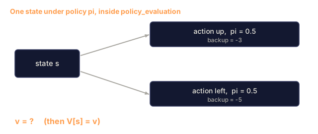
4. Under policy pi a state has {'up': 0.5, 'left': 0.5}. The backup for 'up' is -3 and for 'left' is -5. What does policy_evaluation set v to?Apply
A state s with two action branches under the policy: action up with probability 0.5 and backup -3, and action left with probability 0.5 and backup -5, and the line v equals question mark.
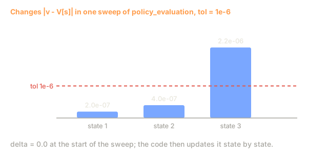
5. In policy_evaluation, the per-state changes in one sweep are 2e-7, 4e-7 and 2.2e-6, and tol is 1e-6. What happens?Apply
Three bars of per-state changes in one sweep (2e-07, 4e-07 and 2.2e-06) against a dashed line at tol = 1e-06, with the bars for states 1 and 2 below the line and state 3 above it.
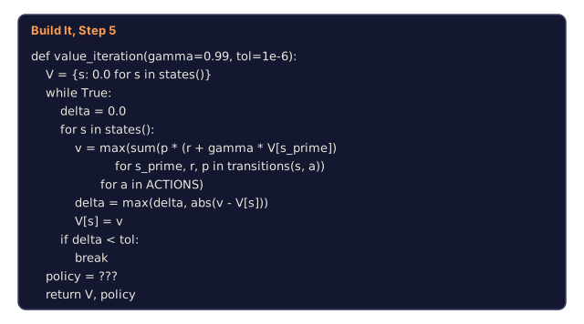
6. After value_iteration's loop breaks, how does the function get its policy?Apply
The lesson's value_iteration function with a loop that updates V with max backups until delta is below tol, then breaks, followed by a line policy = question marks and return V, policy.
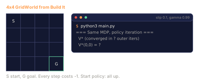
7. Run policy_iteration on the 4x4 GridWorld from the Build It section. What does the lesson say to expect?Apply
A 4x4 grid with S at the top left and G at the bottom right, beside a terminal running main.py for policy iteration where the number of outer iterations and V*(0,0) are question marks, with notes that every step costs -1 and the start policy is all up.

Pitfalls

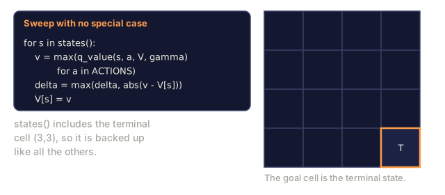
  • Forgetting to handle terminals. If you apply Bellman to an absorbing state, it still picks up a "best action" that changes nothing. Guard with if s == terminal: V[s] = 0.
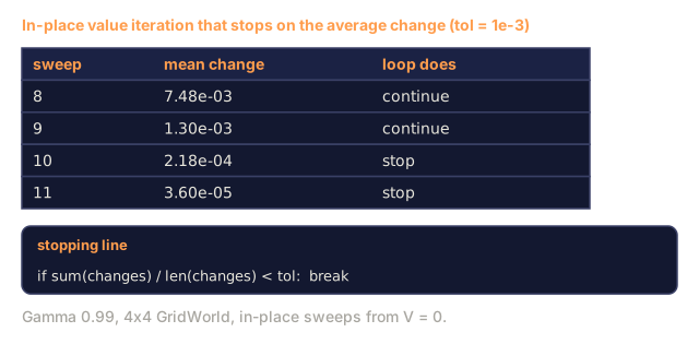
  • Sup-norm vs L2 convergence. Use max |V_new - V|, not average. The theoretical guarantee is on the sup-norm.
  • In-place vs synchronous updates. Updating V[s] in-place (Gauss-Seidel) converges faster than a separate V_new dict (Jacobi). Production code uses in-place.
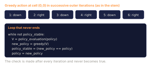
  • Policy ties. If two actions have equal Q-value, argmax may break ties differently each iteration, causing the "policy stable" check to oscillate. Use a stable tie-break (first action in fixed order).
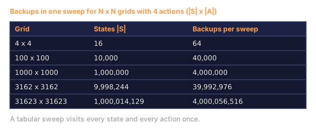
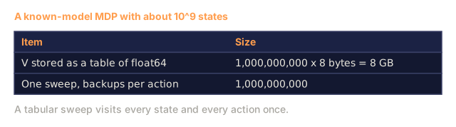
  • State-space explosion. DP is O(|S| · |A|) per sweep. Works up to ~10⁷ states. Beyond that, you need function approximation (Phase 9 · 05 onwards).
Check: Pitfalls0/9
1. What is a synchronous (Jacobi-style) update in dynamic programming?Define
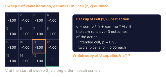
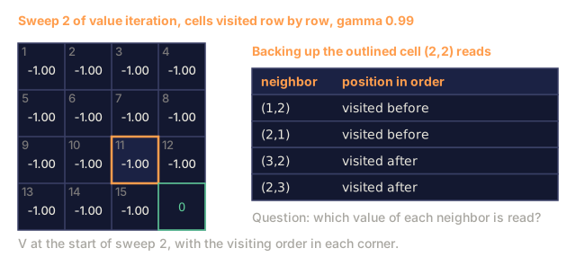
A 4x4 grid of V values at the start of sweep 2 (all -1.00, goal 0) with the order in which cells are visited numbered in each corner and cell (2,2) outlined, beside a table of its four neighbors and whether each is visited before or after it.
Sweep 1 was synchronous here, which is why every non-goal cell starts sweep 2 at -1.00.
2. What is an in-place (Gauss-Seidel-style) update?Define
A 4x4 grid of V values at the start of sweep 2 with visiting order numbers and cell (2,2) outlined, beside a card describing the backup of that cell as a sum over three outcomes (intended cell with probability 0.90, two slip cells with 0.05 each) and the question of which copy of V supplies the successor values.
Sweep 1 was synchronous here, which is why every non-goal cell starts sweep 2 at -1.00.
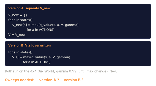
3. Why does the lesson recommend in-place updates over synchronous ones for value iteration in production code?Explain
Two code cards for a value iteration sweep: version A builds a separate V_new dictionary and then assigns V = V_new, version B overwrites V[s] inside the loop, with the sweeps each needs on the 4x4 GridWorld left as question marks.
Sketch of the two sweep bodies (terminal skip omitted), not run as shown.
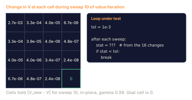
4. Which quantity should the stopping check of a DP sweep use, and why?Explain
A 4x4 grid of the per-cell change in V during sweep 10 of value iteration (values between 0 and about 2.7e-03, goal cell 0), beside a card with tol = 1e-3 and a loop whose stopping statistic is left as three question marks.
Computed with the lesson's value iteration. tol = 1e-3 is chosen for this picture.
5. Why does plain tabular DP stop being practical for very large state spaces?Explain
A table of grid sizes 4x4, 100x100, 1000x1000, 3162x3162 and 31623x31623 with their number of states (16 up to about 10^9) and the number of backups in one sweep with 4 actions (64 up to about 4x10^9).
Computed here.
6. The terminal state's value is being backed up like any other state, as if it had a best action. Which fix does the lesson give?Analyze
A value iteration sweep with no special case for any cell, beside a 4x4 grid with the terminal cell (3,3) at the bottom right outlined, and a note that states() includes the terminal cell and backs it up like the others.
Sketch of the sweep as the stem describes it, typed, not run.
7. Your policy-iteration loop never terminates: the greedy policy toggles between two actions every outer iteration, though both look equally good. What is going on?Analyze
A strip of the greedy action at cell (0,0) over six outer iterations alternating down, right, down, right, down, right, above a sketch of a policy-iteration loop whose stability check never becomes true.
The alternation is the stem's scenario and the loop is a sketch, both typed, not run.
8. A DP loop stops when the average change in V is below tol, yet one state's value is still moving a lot per sweep. Why is that a problem?Analyze
A table of sweeps 8 to 11 of in-place value iteration with the mean change per sweep (7.48e-03, 1.30e-03, 2.18e-04, 3.60e-05) and what a loop stopping on mean change below 1e-3 does (stops at sweep 10), above the stopping line of code.
9. A known-model MDP has about 10^9 states. Which approach fits?Design
A table for 10^9 states: a value table of float64 needs 8 GB and one sweep makes 1,000,000,000 backups per action, with a note that a tabular sweep visits every state and action.
Sizes computed here.

Use It

In 2026, DP is the correctness baseline and the inner loop of planners:

Use caseMethod
Solve a small tabular MDP exactlyValue iteration (simpler) or policy iteration (fewer outer steps)
Verify a Q-learning / PPO implementationCompare to DP-optimal V* on a toy environment
Model-based RL (Phase 9 · 10)Bellman backup on a learned transition model
Planning in AlphaZero / MuZeroMonte Carlo Tree Search = async Bellman backup
Offline RL (CQL, IQL)Conservative Q-iteration: DP with a penalty on OOD actions

Every time someone says "the optimal value function," they mean "the DP fixed point." When you see V* or Q* in a paper, picture this loop.
Check: Use It0/3
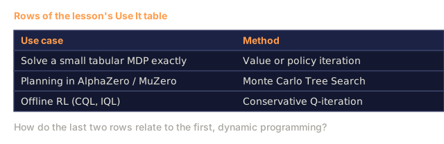
1. How does the Use It table relate MCTS and offline RL methods such as CQL and IQL to dynamic programming?Explain
Three rows taken from the Use It table: solving a small tabular MDP exactly with value or policy iteration, planning in AlphaZero and MuZero with Monte Carlo Tree Search, and offline RL with CQL and IQL with conservative Q-iteration, above a question about how the last two relate to dynamic programming.
Rows from the lesson with the Method text shortened; the relation is left out.
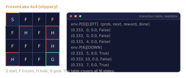
2. You must verify a new PPO implementation on FrozenLake, whose transition table you can read. Which approach fits?Design
The FrozenLake 4x4 map (S F F F / F H F H / F F F H / H F F G) beside two entries of its readable transition table, env.P[0][LEFT] and env.P[6][DOWN], each three outcomes with probability 1/3.
Table built here from the FrozenLake rules in the env.P format.
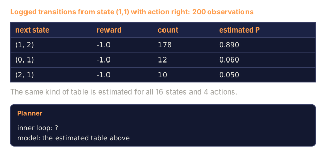
3. You have learned a transition model from data and want to plan with it. What should the planner's inner loop be?Design
A table of 200 logged transitions from state (1,1) with action right giving counts 178, 12 and 10 for the three next states and the estimated probabilities, above a planner card with the inner loop left as a question mark.
Samples drawn here from the lesson's model with a fixed seed.

Ship It

Save as outputs/skill-dp-solver.md:

markdown
---
name: dp-solver
description: Solve a small tabular MDP exactly via policy iteration or value iteration. Report convergence behavior.
version: 1.0.0
phase: 9
lesson: 2
tags: [rl, dynamic-programming, bellman]
---
 
Given an MDP with a known model, output:
 
1. Choice. Policy iteration vs value iteration. Reason tied to |S|, |A|, γ.
2. Initialization. V_0, starting policy. Convergence sensitivity.
3. Stopping. Sup-norm tolerance ε. Expected number of sweeps.
4. Verification. V*(s_0) computed exactly. Greedy policy extracted.
5. Use. How this baseline will be used to debug/evaluate sampling-based methods.
 
Refuse to run DP on state spaces > 10⁷. Refuse to claim convergence without a sup-norm check. Flag any γ ≥ 1 on an infinite-horizon task as a guarantee violation.
Author's Note

The tie-breaking pitfall above cost me an afternoon the first time I wrote policy iteration. My argmax picked whichever action happened to sort first in a dict, and the "has the policy stabilized?" check kept flipping between two equally good policies forever, so the loop never terminated. It looked like a bug in the Bellman equation. It was a five-character sort-order bug. If you ever compare a Q-learning or PPO run against a DP baseline and the numbers refuse to line up, check tie-breaking before you touch the RL code. The policy-stable check only terminates cleanly when the greedy step is deterministic; V* itself doesn't care which tied action you pick.

Exercises

  1. Easy. Run value iteration on the 4×4 GridWorld with γ ∈ {0.9, 0.99}. How many sweeps until max |ΔV| < 1e-6? Print V* as a 4×4 grid.
  2. Medium. Compare policy iteration vs value iteration on the stochastic GridWorld (slip probability 0.1). Count: sweeps, wall-clock time, final V*(0,0). Which converges faster in iterations? In wall-clock?
  3. Hard. Build modified policy iteration: in the evaluation step, run only k sweeps instead of to convergence. Plot V*(0,0) error vs k for k ∈ {1, 2, 5, 10, 50}. What does the curve tell you about the evaluation/improvement tradeoff?

Key Terms

TermWhat people sayWhat it actually means
Policy iteration"DP algorithm"Alternating evaluation (V^π) and improvement (greedy π w.r.t. V^π) until the policy stops changing.
Value iteration"Faster DP"Bellman optimality backup applied in one sweep; converges to V* geometrically.
Bellman operator"The recursion"(T V)(s) = max_a Σ P (r + γ V(s')); a γ-contraction in sup-norm.
Contraction"Why DP converges"Any operator T with ||T x - T y|| ≤ γ ||x - y|| has a unique fixed point.
GPI"Everything is DP"Generalized Policy Iteration: any method driving V and π to mutual consistency.
Synchronous update"Jacobi-style"Use old V throughout a sweep; cleanly analyzable but slower.
In-place update"Gauss-Seidel-style"Use V as it's being updated; converges faster in practice.

Further Reading

Code

Ships With