TAI BUI
Back to curriculum
BuildPython

Temporal Difference — Q-Learning & SARSA

Monte Carlo waits until the episode ends. TD updates after every single step by bootstrapping the next value estimate. Q-learning is off-policy and optimistic; SARSA is on-policy and cautious. Both fit in one line of code, and both underpin every deep-RL method in this phase.

TIME: ~75 minutesPREREQUISITES: Phase 9 · 01 (MDPs), Phase 9 · 02 (Dynamic Programming), Phase 9 · 03 (Monte Carlo)

Learning Objectives

  • State the TD(0) update and the Robbins-Monro conditions its step size needs to converge, and check a learned Q-table against the dynamic-programming ground truth from Lesson 02.
  • Implement Q-learning and SARSA from a shared code skeleton, and explain how the one-line difference between their targets makes one off-policy and the other on-policy.
  • Predict how Q-learning's off-policy max and SARSA's on-policy sample produce different policies on cliff-walking, and place Expected SARSA and n-step TD/TD(λ) on the spectrum between one-step TD and Monte Carlo.
  • Diagnose the recurring TD training pitfalls, maximization bias, Q-value initialization, a GLIE-compliant α/ε schedule, and non-terminating episodes, before they surface as bugs.

The Problem

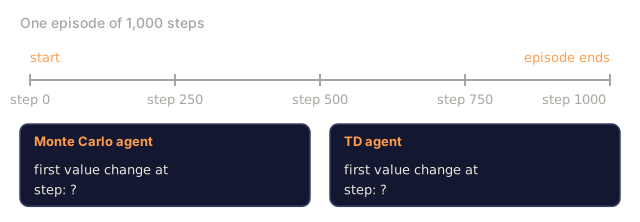
Monte Carlo works, but it makes two expensive demands: it needs episodes that terminate, and it won't update anything until the final return is in. Run a 1,000-step episode and MC waits all 1,000 steps before touching a single value. That's high-variance, low-bias, and slow in practice.

Dynamic programming has the opposite profile. Its backups are zero-variance and bootstrapped, but only because it assumes a known model of the environment, which most real problems don't hand you.

Temporal difference (TD) learning splits the difference. From a single transition (s, a, r, s'), form a one-step target r + γ V(s') and nudge V(s) toward it. No model needed. No complete episodes needed. You do pick up bias from using an approximate V on the right-hand side, but variance drops dramatically compared to MC, and updates start from step one.

This is the pivot modern RL turns on: DQN, A2C, PPO, SAC, all of it. The rest of Phase 9 is layers of function approximation and tricks stacked on top of the one-step TD update you're about to write in this lesson.
Warm-up0/3
1. In an MDP, what does a discount factor gamma below 1 do to rewards that arrive later?Warm-up
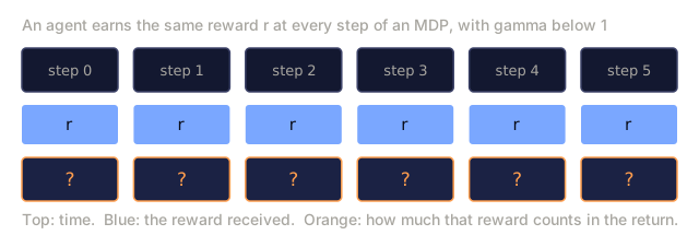
Six time steps, step 0 to step 5, each with the same reward r in a blue bar of equal height and an orange box with a question mark for the weight that reward gets in the return, with gamma below 1.
2. Dynamic programming methods such as value iteration can compute optimal values. What do they need that many real problems do not provide?Warm-up
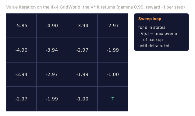
A 4x4 grid of optimal state values from value iteration with gamma 0.99 and reward -1 per step: -5.85 at the top-left start cell down to -1.00 beside the terminal cell, next to a four-line sweep loop for value iteration.
Computed here with value iteration on the lesson's GridWorld.
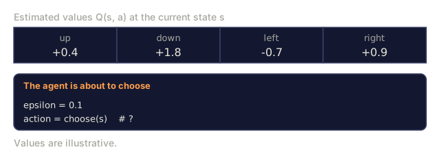
3. What does an epsilon-greedy policy do when choosing an action?Warm-up
Four action cells with estimated values up +0.4, down +1.8, left -0.7 and right +0.9, above a card saying epsilon = 0.1 and action = choose(s) with a question mark.
Check: The Problem0/1
1. Why does Monte Carlo update slowly compared with TD, especially on long episodes?Explain
A timeline of one 1,000-step episode with ticks at steps 0, 250, 500, 750 and 1000 and two cards, Monte Carlo agent and TD agent, each asking at which step the first value change happens, marked with a question mark.

The Concept

Q-learning vs SARSA: off-policy max vs on-policy Q(s', a')

The TD(0) update for V:

V(s) ← V(s) + α [r + γ V(s') - V(s)]

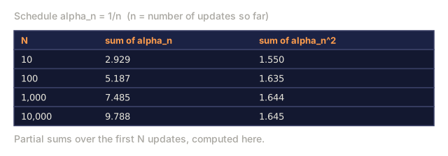
The bracketed quantity is the TD error, δ = r + γ V(s') - V(s), the online analogue of G_t - V(s_t) in MC. Convergence needs α to satisfy the Robbins-Monro conditions (Σ α = ∞, Σ α² < ∞) with every state visited infinitely often.

Q-learning. An off-policy TD method for control:

Q(s, a) ← Q(s, a) + α [r + γ max_{a'} Q(s', a') - Q(s, a)]

The max assumes the greedy policy gets followed from s' onward, no matter what action the agent actually takes. That decoupling is what lets Q-learning learn Q* while the agent keeps exploring via ε-greedy. Mnih et al. (2015) turned this exact idea into deep Q-learning on Atari (Lesson 05).

SARSA. An on-policy TD method:

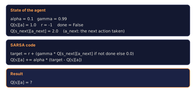
Q(s, a) ← Q(s, a) + α [r + γ Q(s', a') - Q(s, a)]

The name comes from the tuple it consumes: (s, a, r, s', a'). SARSA plugs in the action a' the agent actually takes next, not the greedy argmax. It converges to Q^π for whatever ε-greedy π is currently running, which becomes Q* only in the limit ε → 0.

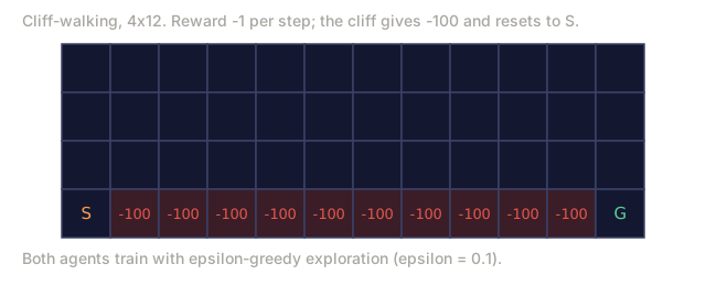
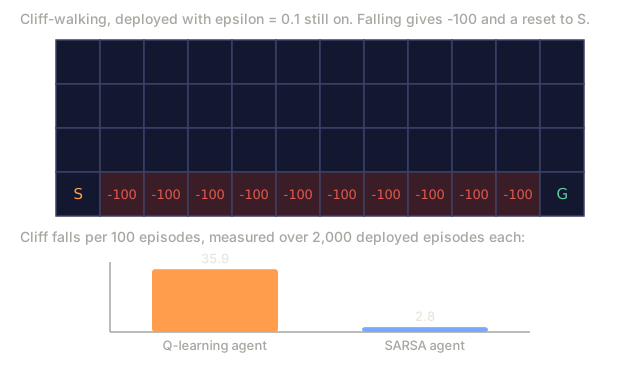
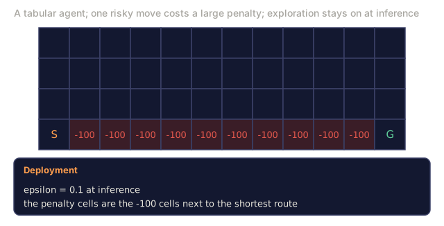
The cliff-walking difference. On the classic cliff-walking task, where falling off the cliff costs a reward of -100, Q-learning learns the optimal path right along the cliff edge and occasionally eats the penalty during exploration. SARSA learns a safer path one step back from the edge, because it bakes exploration noise directly into its Q-value. Train both long enough and they converge to the same optimum as ε → 0. What matters in practice is deployment: if exploration is still happening once the agent goes live, SARSA's caution shows.

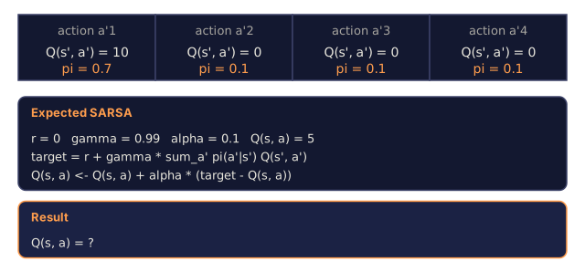
Expected SARSA. Replace Q(s', a') with its expected value under π:

Q(s, a) ← Q(s, a) + α [r + γ Σ_{a'} π(a'|s') Q(s', a') - Q(s, a)]

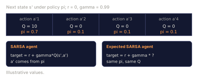
Lower variance than SARSA, since there's no sample of a' to add noise, with the same on-policy target. It's the default in most modern textbooks for that reason.

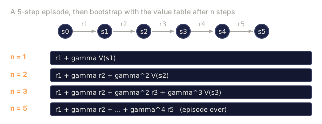
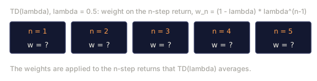
n-step TD and TD(λ). You can interpolate between TD(0) and MC just by waiting n steps before bootstrapping: n=1 is TD, n=∞ is MC. TD(λ) averages over every n with geometric weights (1-λ)λ^{n-1}. Most deep RL sits somewhere between n=3 and n=20.
Check: The Concept0/15
1. What does TD(0) do?Define
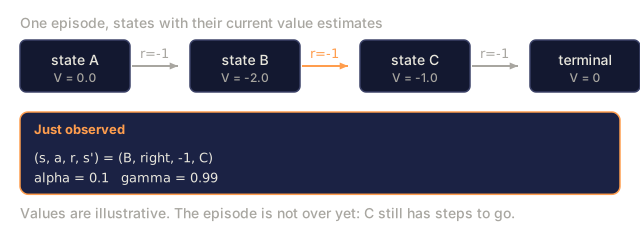
A chain of states A, B, C and a terminal state with current value estimates 0.0, -2.0, -1.0 and 0, rewards of -1 on each arrow, and a card for the transition just observed, (B, right, -1, C), with alpha 0.1 and gamma 0.99.
2. In TD(0), what does the quantity delta = r + gamma V(s') - V(s) measure?Define
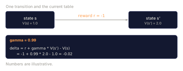
Two states, s with V(s) = 1.0 and s' with V(s') = 2.0, joined by an arrow with reward r = -1, and a card with gamma 0.99 evaluating delta = r + gamma V(s') - V(s) as -0.02.
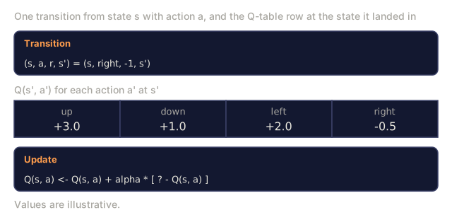
3. What is Q-learning?Define
A transition (s, right, -1, s'), the Q-table row at s' with up +3.0, down +1.0, left +2.0 and right -0.5, and an update line with the target left as a question mark.
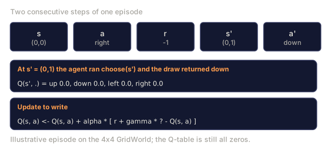
4. What does SARSA use as the next-state term in its target, and what does it learn?Define
Five boxes for one transition on the GridWorld, s = (0,0), a = right, r = -1, s' = (0,1) and a' = down, a card saying choose at s' returned down while the Q-table is all zeros, and an update line with the next-state term left as a question mark.
5. Expected SARSA replaces the sampled Q(s', a') in the SARSA update with what?Define
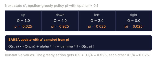
Four action cells at the next state with Q values up 1.0, down 4.0, left 2.0, right 0.0 and epsilon-greedy probabilities 0.025, 0.925, 0.025, 0.025, above a SARSA update line with the next-state term shown as a question mark.
6. What is bootstrapping in TD learning?Define
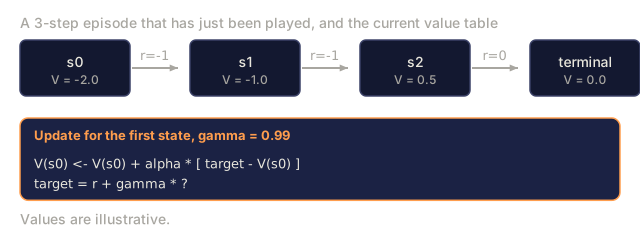
A three-step episode s0, s1, s2, terminal with current values -2.0, -1.0, 0.5 and 0 and rewards -1, -1, 0, and a card for the update of V(s0) whose target r + gamma * ? has the next-state term left as a question mark.
7. Why can Q-learning learn Q* even though the agent keeps exploring with epsilon-greedy?Explain
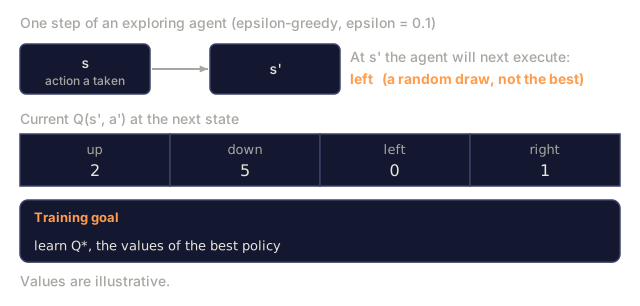
A step from s to s' by an exploring agent, a note that the agent will next execute left as a random draw, and the Q row at s' with up 2, down 5, left 0, right 1, above a card with the goal of learning Q*.
8. Why does SARSA with a fixed epsilon learn Q^pi rather than Q*?Explain
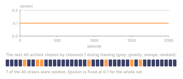
A flat line at epsilon 0.1 over 2000 episodes, and a strip of 40 consecutive actions from choose(s') coloured grey for greedy and orange for random, 7 of them random.
Draws simulated with numpy (seed 5).
9. On cliff-walking, how do the policies learned by Q-learning and SARSA differ?Explain
A cliff-walking grid of 4 rows by 12 columns with start S at the bottom left, goal G at the bottom right and the ten cells between them marked -100 as the cliff, reward -1 per step.
Standard cliff layout: the cliff fills the bottom row between S and G.
10. Why does Expected SARSA have lower variance than SARSA while keeping the same on-policy target?Explain
Four next-state actions with Q values 10, 0, 0, 0 and policy probabilities 0.7, 0.1, 0.1, 0.1 with r = 0 and gamma 0.99, above two cards: a SARSA agent whose target uses a sampled a' from pi, and an Expected SARSA agent whose target term is a question mark.
11. How does n-step TD relate to TD(0) and Monte Carlo, and what does TD(lambda) add?Explain
A five-step episode s0 to s5 with rewards r1 to r5, and four target formulas for n = 1, 2, 3 and 5: the first n rewards, discounted, followed by gamma^n times the value of state s_n, except n = 5 which ends at the terminal state with no value term.
12. What do the Robbins-Monro conditions require of the step size alpha for TD(0) to converge?Explain
A table of partial sums for the step-size schedule alpha_n = 1/n at N = 10, 100, 1,000 and 10,000: the sum of alpha_n is 2.929, 5.187, 7.485, 9.788 and the sum of alpha_n squared is 1.550, 1.635, 1.644, 1.645.
13. Under pi the next-state action probabilities are 0.7, 0.1, 0.1, 0.1 with Q(s', .) = 10, 0, 0, 0. With r=0, gamma=0.99, alpha=0.1 and Q(s, a)=5, what does the Expected SARSA update give?Apply
Four next-state actions with Q values 10, 0, 0, 0 and policy probabilities 0.7, 0.1, 0.1, 0.1, and a card with r 0, gamma 0.99, alpha 0.1, Q(s, a) 5 and the Expected SARSA update, with the result left as Q(s, a) = ?.
14. For TD(lambda) with lambda=0.5, what weight does the n=3 step return get under the weights (1-lambda) lambda^(n-1)?Apply
Five cards for n = 1 to 5, each showing a question mark for the weight of the n-step return under TD(lambda) with lambda 0.5 and weights (1 - lambda) * lambda^(n-1).
15. Both agents are trained on cliff-walking and deployed with epsilon still 0.1. The Q-learning agent falls off the cliff more often than the SARSA agent. Why?Analyze
The cliff-walking grid with the cliff cells marked -100, and two bars of falls per 100 deployed episodes with epsilon still 0.1: Q-learning agent 35.9, SARSA agent 2.8.
Standard cliff layout: the cliff fills the bottom row between S and G. Trained here with numpy (500 episodes, epsilon 0.1, alpha 0.5, gamma 1, seed 1; the lesson gives no cliff hyperparameters). Falls counted over 2,000 deployed episodes.

Build It

Step 1: SARSA on ε-greedy policy

python
def sarsa(env, episodes, alpha=0.1, gamma=0.99, epsilon=0.1):
    Q = defaultdict(lambda: {a: 0.0 for a in ACTIONS})
 
    def choose(s):
        if random() < epsilon:
            return choice(ACTIONS)
        return max(Q[s], key=Q[s].get)
 
    for _ in range(episodes):
        s = env.reset()
        a = choose(s)
        while True:
            s_next, r, done = env.step(s, a)
            a_next = choose(s_next) if not done else None
            target = r + (gamma * Q[s_next][a_next] if not done else 0.0)
            Q[s][a] += alpha * (target - Q[s][a])
            if done:
                break
            s, a = s_next, a_next
    return Q

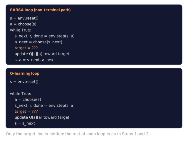
Eight lines, and the only difference from Q-learning is the target line.

Step 2: Q-learning

python
def q_learning(env, episodes, alpha=0.1, gamma=0.99, epsilon=0.1):
    Q = defaultdict(lambda: {a: 0.0 for a in ACTIONS})
    for _ in range(episodes):
        s = env.reset()
        while True:
            a = choose(s, Q, epsilon)
            s_next, r, done = env.step(s, a)
            target = r + (gamma * max(Q[s_next].values()) if not done else 0.0)
            Q[s][a] += alpha * (target - Q[s][a])
            if done:
                break
            s = s_next
    return Q

The max decouples target from behavior. That single symbol is the whole difference between on-policy and off-policy.

Step 3: learning curves

Track mean return per 100 episodes. Q-learning converges faster on the simple deterministic GridWorld; SARSA is the more conservative learner on cliff-walking. On the 4×4 GridWorld in code/main.py, both land near-optimal after roughly 2,000 episodes at α=0.1, ε=0.1.

Step 4: compare to DP truth

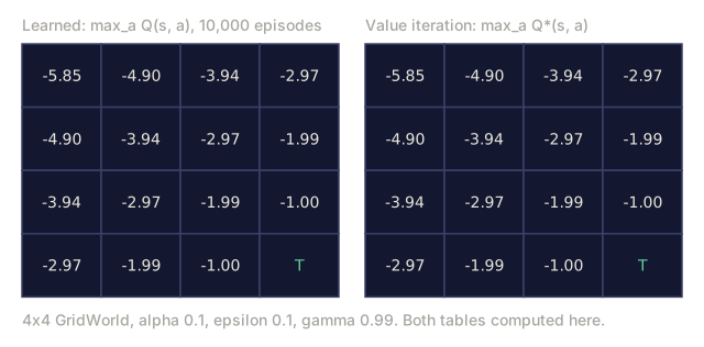
Run value iteration (Lesson 02) to get Q*, then check max_{s,a} |Q_learned(s,a) - Q*(s,a)|. A healthy tabular TD agent lands within ~0.5 of Q* on the 4×4 GridWorld after 10,000 episodes.
Check: Build It0/6
1. Which single difference between the Q-learning and SARSA updates makes one off-policy and the other on-policy?Explain
Two loop skeletons side by side, SARSA (reset, choose, step, choose next action, target, update, advance both s and a) and Q-learning (reset, choose, step, target, update, advance s), each with its target line replaced by ???.
2. How does the lesson check that a learned Q-table is correct on the small GridWorld?Explain
Two 4x4 grids of state values side by side: the best Q-value per state learned by Q-learning after 10,000 episodes, and the best Q* value per state from value iteration, with the terminal corner marked T.
Q-learning run with the lesson's code (seed 2).
3. With alpha=0.1 and gamma=0.99, Q[s][a]=1.0, r=-1, a non-terminal step, and Q[s_next][a_next]=2.0 for the next action taken, what does the SARSA code set Q[s][a] to?Apply
A card with alpha 0.1, gamma 0.99, Q[s][a] 1.0, r -1, done False and Q[s_next][a_next] 2.0, the two SARSA code lines for target and update, and a result card Q[s][a] = ?.
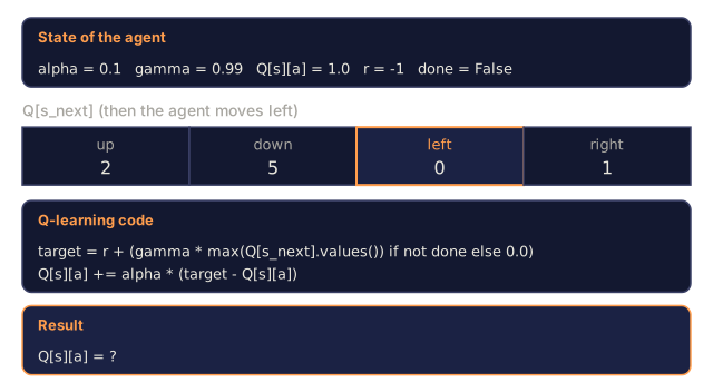
4. With alpha=0.1, gamma=0.99, Q[s][a]=1.0 and r=-1, the next state has Q values up 2.0, down 5.0, left 0.0, right 1.0 and the agent then moves left. What does the Q-learning code set Q[s][a] to?Apply
The state of the agent (alpha 0.1, gamma 0.99, Q[s][a] 1.0, r -1), the row Q[s_next] with up 2, down 5, left 0, right 1 and left outlined as the move that follows, the two Q-learning code lines and a result card Q[s][a] = ?.
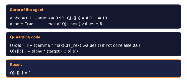
5. With alpha=0.1, gamma=0.99, Q[s][a]=4.0 and r=10, the step ends the episode (done=True) and the next state's Q values go up to 8. What does the code set Q[s][a] to?Apply
A card with alpha 0.1, gamma 0.99, Q[s][a] 4.0, r 10, done True and a maximum of 8 among the next state's Q values, the Q-learning target and update code lines, and a result card Q[s][a] = ?.
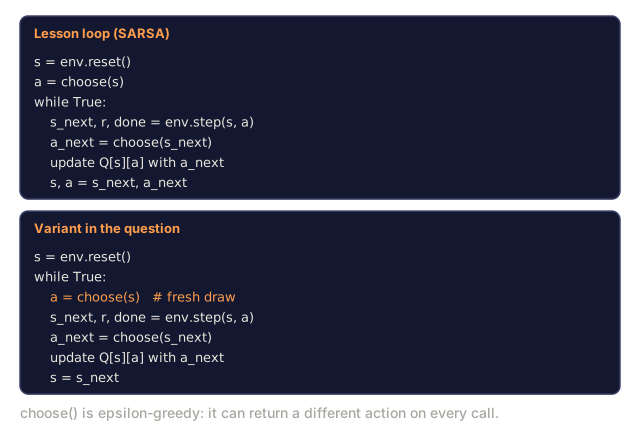
6. In the SARSA loop, a_next is chosen before the update and becomes a on the next step. What would change if the loop instead drew a fresh action at the top of each step?Apply
Two SARSA loops side by side: the lesson's, which picks a once before the loop and sets a to a_next at the end, and a variant that calls a = choose(s) at the top of each step and only sets s = s_next at the end.

Pitfalls

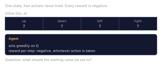
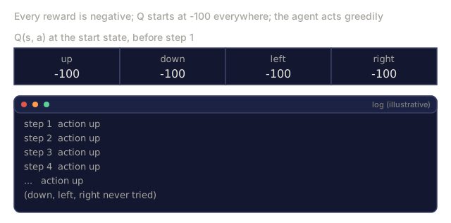
  • Initial Q values matter. Optimistic init (Q = 0 for a negative-reward task) encourages exploration. Pessimistic init can trap a greedy policy forever.
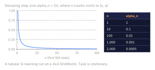
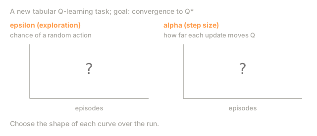
  • α schedule. Constant α is fine for non-stationary problems. Decaying α_n = 1/n gives convergence in theory, but it's too slow in practice, so pin α in [0.05, 0.3] and watch the learning curve instead.
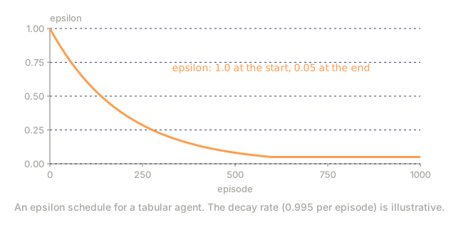
  • ε schedule. Start high (ε=1.0) and decay to ε=0.05. "GLIE" (greedy in the limit with infinite exploration) is the convergence condition you're aiming for.
  • Max bias in Q-learning. The max operator is biased upward whenever Q is noisy, which leads to overestimation. Hasselt's Double Q-learning (used by DDQN in Lesson 05) fixes this with two Q tables.
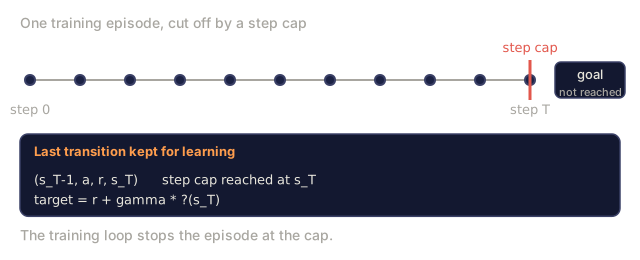
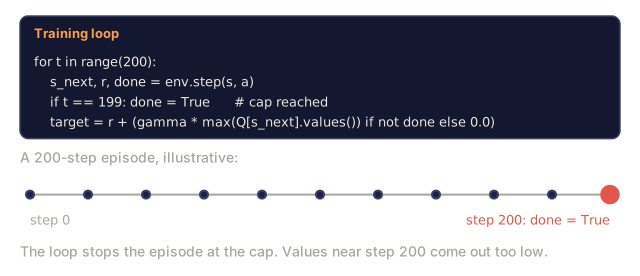
  • Non-terminating episodes. TD can learn without terminals, but you need to either cap steps or handle the bootstrap correctly at the cap. The standard move: treat the cap as non-terminal and keep bootstrapping.
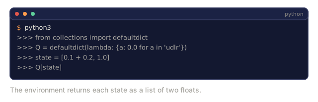
  • State hashing. If states are tuples or tensors, use a hashable key: a tuple, not a list, and floats rounded rather than raw.
Check: Pitfalls0/10
1. What does GLIE stand for, and what role does it play for the epsilon schedule?Define
A line chart of epsilon over 1000 episodes falling from 1.0 at episode 0 to a floor of 0.05, with a note that the decay rate of 0.995 per episode is illustrative.
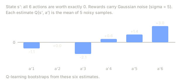
2. What causes maximization bias in Q-learning, and how is it fixed?Define
Six bars for the estimated values of 6 actions at one state whose true values are all 0, each the mean of 5 samples with Gaussian noise of sigma 5, so the bars scatter above and below zero, and a note that Q-learning bootstraps from these estimates.
Samples drawn here with numpy (seed 3).
3. How do initial Q values affect exploration on a task with negative rewards?Explain
One state with four untried actions, each with a question mark as its initial Q value, and a card saying the agent acts greedily and every reward is negative.
4. What step-size advice does the lesson give for practice, compared with the theoretical schedule?Explain
A curve of alpha_n = 1/n for the first 100 visits, falling from 1 to 0.01, and a table of its values: 1 at n = 1, 0.1 at 10, 0.01 at 100, 0.001 at 1,000 and 0.0005 at 2,000.
5. When an episode is cut off by a step cap, how should the TD update treat the final state?Explain
A timeline of one training episode ending at a step cap before the goal is reached, and a card with the last transition (s_T-1, a, r, s_T), where the step cap is reached at s_T, and a target whose next-state term is a question mark.
6. When states are tuples or tensors, how should they be turned into Q-table keys?Explain
A Python session that builds a defaultdict Q-table, sets state to the list [0.1 + 0.2, 1.0] and then indexes Q[state], with no output shown yet.
The environment returns states as lists of floats.
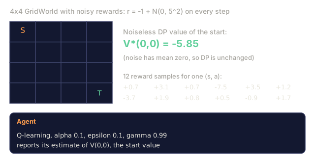
7. On a GridWorld with Gaussian noise added to every reward, a Q-learning agent's value at the start state ends up well above the DP value. What is the most likely cause?Analyze
A 4x4 GridWorld with start S at the top left whose rewards are -1 plus Gaussian noise of standard deviation 5, with the noiseless DP value of the start, V*(0,0) = -5.85, 12 sampled rewards for one state-action pair, and a card describing a Q-learning agent with alpha 0.1 and epsilon 0.1.
Rewards sampled here with numpy (seed 1).
8. Every reward is negative, Q starts at -100 everywhere, and the agent acts greedily. It repeats the first action it tried and never tries others. What fix does the lesson's init advice suggest?Analyze
A Q row at the start state with all four actions at -100, and a log of steps 1 to 4 and onward where the agent always chooses up, with down, left and right never tried.
9. Episodes are capped at 200 steps and the code marks the cap as done, so the target is just r. Values for states reached near the cap come out too low. What is the bug?Analyze
A training loop in which done is forced True at the 200-step cap and the target is r + gamma * max(...) if not done else 0.0, above a timeline of a 200-step episode that is stopped by the cap.
10. You must pick epsilon and alpha schedules for a new tabular Q-learning task and care about convergence. Which plan fits the lesson?Design
Two empty chart frames with question marks, epsilon (chance of a random action) and alpha (how far each update moves Q), against episodes, for a new tabular Q-learning task that must converge.

Use It

The 2026 TD landscape:

TaskMethodReason
Small tabular environmentsQ-learningLearns optimal policy directly.
On-policy safety-criticalSARSA / Expected SARSAConservative during exploration.
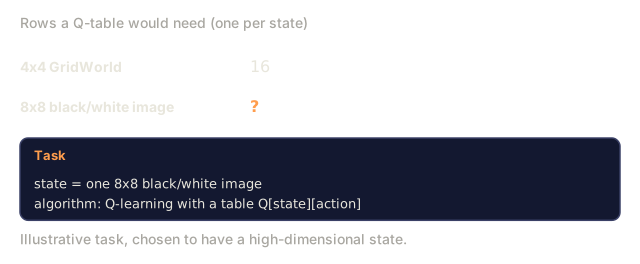
High-dimensional stateDQN (Phase 9 · 05)Neural-net Q-function with replay and target net.
Continuous actionsSAC / TD3 (Phase 9 · 07)TD update on a Q-network; policy net emits actions.
LLM RL (reward-model-based)PPO / GRPO (Phase 9 · 08, 12)Actor-critic with TD-style advantage via GAE.
Offline RLCQL / IQL (Phase 9 · 08)Q-learning with conservative regularization.

Ninety percent of the "RL" you'll read about in 2026 papers is some elaboration of Q-learning or SARSA. Get the tabular update into your fingers before you go looking for the fancier version.
Check: Use It0/2
1. Why does the Use It table send high-dimensional state tasks to DQN rather than a tabular method?Explain
A row count for a table-based Q-learning agent: 16 for the 4x4 GridWorld and a question mark for a task whose state is one 8x8 black and white image, with a card describing that task.
2. You will deploy a tabular agent on a task with a large penalty for a risky move, and exploration stays on at inference. Which method fits, and why?Design
The cliff-walking grid with the ten cliff cells marked -100 along the shortest route, and a card saying the agent keeps epsilon 0.1 at inference.
Cliff-walking stands in for the task's risky move. Standard layout: cliff fills the bottom row between S and G.

Ship It

Save as outputs/skill-td-agent.md:

markdown
---
name: td-agent
description: Pick between Q-learning, SARSA, Expected SARSA for a tabular or small-feature RL task.
version: 1.0.0
phase: 9
lesson: 4
tags: [rl, td-learning, q-learning, sarsa]
---
 
Given a tabular or small-feature environment, output:
 
1. Algorithm. Q-learning / SARSA / Expected SARSA / n-step variant. One-sentence reason tied to on-policy vs off-policy and variance.
2. Hyperparameters. α, γ, ε, decay schedule.
3. Initialization. Q_0 value (optimistic vs zero) and justification.
4. Convergence diagnostic. Target learning curve, `|Q - Q*|` check if DP is possible.
5. Deployment caveat. How will exploration behave at inference? Is SARSA's conservatism needed?
 
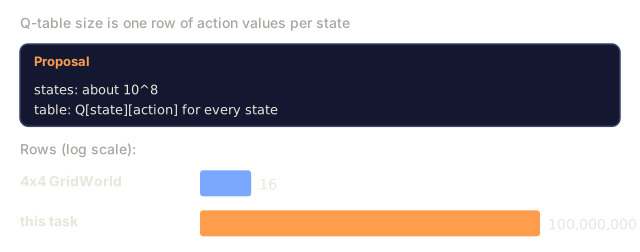
Refuse to apply tabular TD to state spaces > 10⁶. Refuse to ship a Q-learning agent without a max-bias caveat. Flag any agent trained with ε held at 1.0 throughout (no exploitation phase).
Check: Ship It0/1
1. A task has about 10^8 states and a teammate proposes a tabular Q-table. What do you do?Design
A proposal card of about 10^8 states with a Q table indexed by state and action, and two log-scale bars of rows needed: 16 for the 4x4 GridWorld and 100,000,000 for this task.

Exercises

  1. Easy. Implement Q-learning and SARSA on the 4×4 GridWorld. Plot learning curves (mean return per 100 episodes) for 2,000 episodes. Who converges faster?
  2. Medium. Build a cliff-walking environment (4×12, last row is the cliff with reward -100 and reset to start). Compare Q-learning and SARSA final policies. Screenshot the paths each takes. Which is closer to the cliff?
  3. Hard. Implement Double Q-learning. On a noisy-reward GridWorld (Gaussian noise σ=5 added to per-step reward), show Q-learning overestimates V*(0,0) by a meaningful amount while Double Q-learning does not.

Key Terms

TermWhat people sayWhat it actually means
TD error"The update signal"δ = r + γ V(s') - V(s), the bootstrapped residual.
TD(0)"One-step TD"Update after every transition using only the next state's estimate.
Q-learning"Off-policy RL 101"TD update with max over next-state actions; learns Q* regardless of behavior policy.
SARSA"On-policy Q-learning"TD update using the actual next action; learns Q^π for current ε-greedy π.
Expected SARSA"The low-variance SARSA"Replace sampled a' with its expectation under π.
GLIE"Correct exploration schedule"Greedy in the Limit with Infinite Exploration; needed for Q-learning convergence.
Bootstrapping"Using current estimate in the target"What distinguishes TD from MC. Source of bias but massive variance reduction.
Maximization bias"Q-learning overestimates"max over noisy estimates is upward-biased; fixed by Double Q-learning.

Further Reading

Code

Ships With