TAI BUI
Back to curriculum
BuildPython

Actor-Critic — A2C and A3C

REINFORCE is noisy. Add a critic that learns `V̂(s)`, subtract it from the return, and what's left is an advantage: same expectation, far lower variance. That's actor-critic. A2C runs it synchronously; A3C runs it across threads. Both give you the mental model behind every modern deep-RL method.

TIME: ~75 minutesPREREQUISITES: Phase 9 · 04 (TD Learning), Phase 9 · 06 (REINFORCE)

Learning Objectives

  • Explain why subtracting a learned V̂(s_t) baseline from the return turns REINFORCE into actor-critic, and why that advantage has the same expectation but far lower variance.
  • Distinguish MC advantage, TD advantage (the TD residual), n-step advantage, and GAE(λ), and place each on the bias/variance spectrum.
  • Implement a critic update and a GAE-based advantage/return calculation in code, and combine them with a policy-gradient actor update into one on-policy training step.
  • Contrast A2C's synchronous batched rollout with A3C's asynchronous worker-thread design, and place actor-critic in the lineage of PPO, IMPALA, SAC, GRPO, and DPO.

The Problem

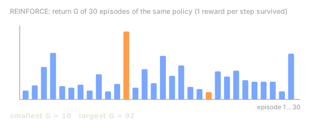
Vanilla REINFORCE works, but its variance is terrible. Monte Carlo returns G_t can swing over a factor of 10 between episodes. Multiply that noise by ∇ log π and average it, and you get a gradient estimator that needs thousands of episodes to move the policy the same distance a handful of DQN updates would.

The variance comes from using raw returns. Subtract a baseline b(s_t) (any function of state, including a learned value) and the expectation stays the same while the variance drops. The best tractable baseline is V̂(s_t). Now the quantity multiplying ∇ log π is the advantage:

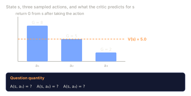
A(s, a) = G - V̂(s)

An action is good if it produced above-average return, bad if below. REINFORCE with a learned critic is actor-critic. The critic gives the actor a low-variance teacher, and that pairing is every deep-policy method after 2015: A2C, A3C, PPO, SAC, IMPALA.
Warm-up0/3
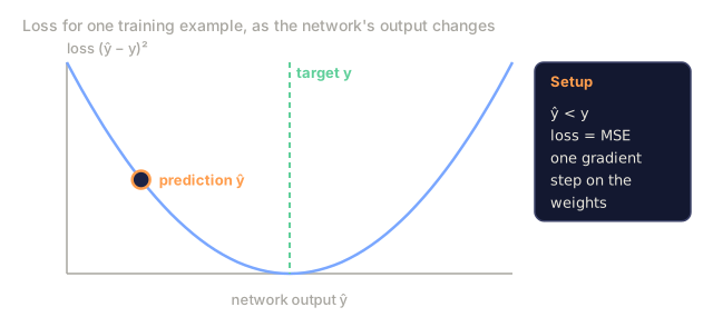
1. A network predicts a number and is trained by minimizing mean squared error. If a prediction is below its target, what does one gradient step do?Warm-up
A parabola of squared-error loss against the network output with a dashed vertical line at the target and an orange dot on the curve at a prediction left of (below) the target; a side card says the prediction is below the target, the loss is MSE, and one gradient step is taken on the weights.
Schematic: the axis has no numbers because the stem gives none.
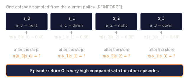
2. In REINFORCE, what does a gradient step do to the probability of the actions taken in an episode that earned a very high return?Warm-up
Four steps of one sampled episode, each with its state, the chosen action and the policy probability of that action (0.40, 0.50, 0.30, 0.60), a row of question marks for the probabilities after the gradient step, and a banner saying the episode return is very high.
Probabilities are illustrative.
3. In reinforcement learning, what is the discount factor γ used for?Warm-up
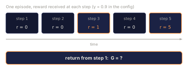
Five time steps with rewards 0, 0, 1, 0 and 5, labelled with a discount factor of 0.9, and a box asking for the return from step 1 as G equals a question mark.
Rewards are illustrative.
Check: The Problem0/4
1. What does the advantage A(s, a) measure?Define
Bars of the return after three sampled actions from one state: a1 with G = 8, a2 with G = 5 and a3 with G = 2, with a dashed line at the critic estimate V-hat(s) = 5.0 and a card asking for A(s, a) of each action.
Values are illustrative.
2. What single change turns REINFORCE into actor-critic?Explain
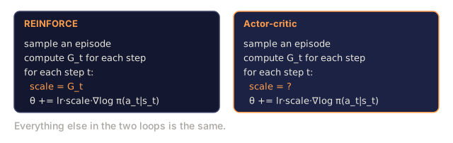
Two pseudocode cards side by side. REINFORCE samples an episode, computes G_t and updates theta by lr times scale times grad log pi with scale equal to G_t. The actor-critic card is identical except that the line scale is a question mark.
Pseudocode, not captured from a run.
3. Why does vanilla REINFORCE produce high-variance gradients?Explain
Bars of the return G of 30 simulated episodes of one policy, ranging from 10 to 92, with the smallest and the largest episode in orange.
Toy simulation with numpy: each episode lasts at least 10 steps, then ends with probability 0.04 per step; reward 1 per step. Illustrative environment.
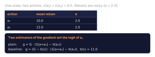
4. Why is subtracting a baseline b(s_t) from the return safe for the policy gradient?Explain
A one-state, two-action problem with equal policy probabilities 0.5 and noisy returns of mean 10.0 and 12.0 and standard deviation 2.0, and two gradient estimators written out: plain G times the score, and (G minus b(s)) times the score with b(s) equal to 11.0.
Toy problem for illustration.

The Concept

Actor-critic: policy net plus value net, TD residual as advantage

Two networks, one shared loss:

  • Actor π_θ(a | s): the policy. Sampled to act. Trained with policy gradient.
  • Critic V_φ(s): estimates expected return from state. Trained to minimize (V_φ(s) - target)².

The advantage. Two standard forms:

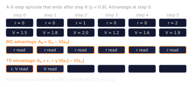
  • MC advantage: A_t = G_t - V_φ(s_t). Unbiased, higher variance.
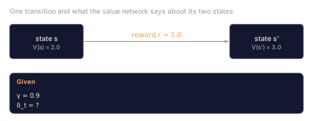
  • TD advantage: A_t = r_{t+1} + γ V_φ(s_{t+1}) - V_φ(s_t). Biased (uses V_φ), far lower variance. Also called the TD residual δ_t.

n-step advantage. Interpolate between the two:

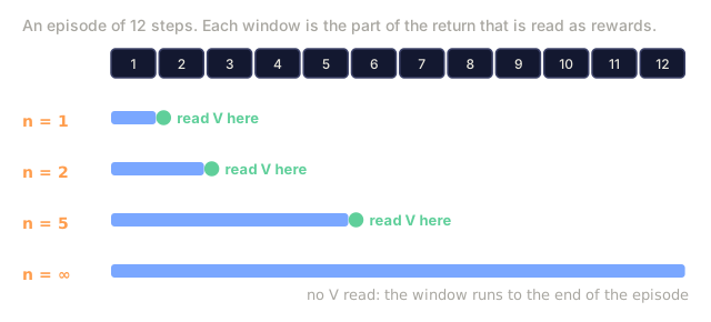
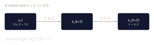
A_t^{(n)} = r_{t+1} + γ r_{t+2} + … + γ^{n-1} r_{t+n} + γ^n V_φ(s_{t+n}) - V_φ(s_t)

n = 1 is pure TD. n = ∞ is MC. Most implementations use n = 5 for Atari, n = 2048 for PPO on MuJoCo.

Generalized Advantage Estimation (GAE). Schulman et al. (2016) proposed an exponentially weighted average over all n-step advantages:

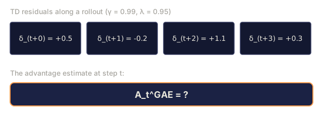
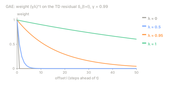
A_t^{GAE} = Σ_{l=0}^{∞} (γλ)^l δ_{t+l}

with λ ∈ [0, 1]. λ = 0 is TD (low variance, high bias). λ = 1 is MC (high variance, unbiased). λ = 0.95 is the 2026 default. Tune it until the bias/variance dial sits where you want.

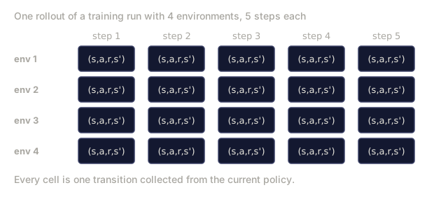
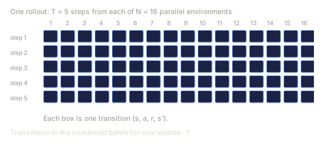
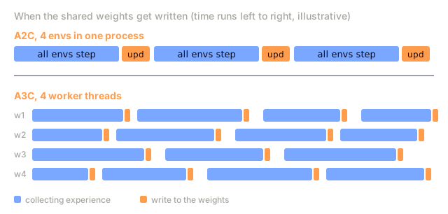
A2C: synchronous advantage actor-critic. Collect T steps across N parallel environments. Compute advantages for each step. Update actor and critic on the combined batch. Repeat. The simpler, more scalable sibling of A3C.

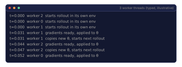
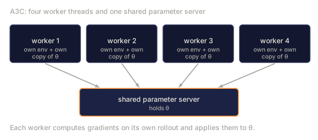
A3C: asynchronous advantage actor-critic. Mnih et al. (2016). Spawn N worker threads, each running an env. Each worker computes gradients locally on its own rollout, then asynchronously applies them to a shared parameter server (one central copy of the weights every worker reads from and writes to). No replay buffer needed: workers decorrelate by running different trajectories. A3C proved you could train on CPUs at scale. In 2026, GPU-based A2C (batched parallel envs) dominates, because GPUs want large batches.

The combined loss.

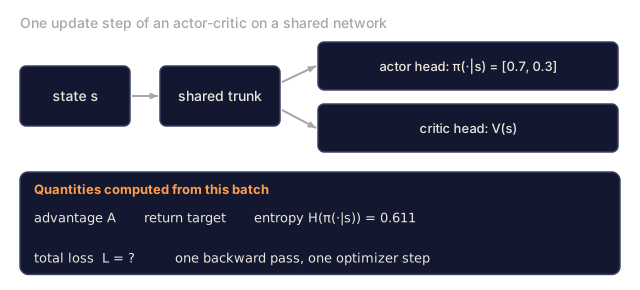
L(θ, φ) = -E[ A_t · log π_θ(a_t | s_t) ] + c_v · E[(V_φ(s_t) - G_t)²] - c_e · E[H(π_θ(·|s_t))]

Three terms: policy-gradient loss, value regression, entropy bonus. c_v ~ 0.5, c_e ~ 0.01 are canonical starting points.
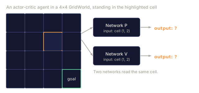
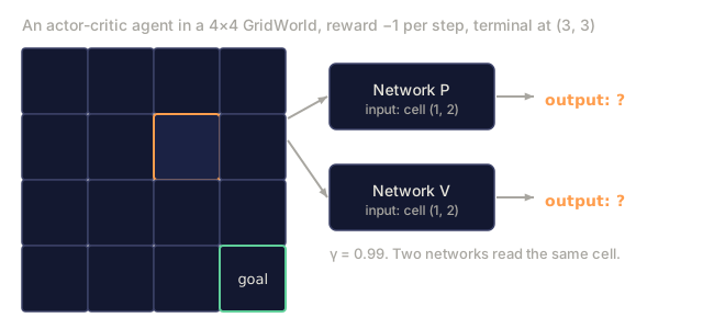
Check: The Concept0/16
1. In an actor-critic method, what is the actor?Define
A 4 by 4 GridWorld with the agent in cell (1, 2) and the goal at (3, 3). Two boxes named Network P and Network V each take that cell as input, and each has an output marked with a question mark.
Schematic of an actor-critic setup; the outputs are hidden.
2. What does the critic V_φ(s) do in actor-critic?Define
A 4 by 4 GridWorld with reward minus 1 per step, gamma 0.99, the agent in cell (1, 2) and the terminal cell at (3, 3). Two boxes named Network P and Network V each take that cell as input, and each has an output marked with a question mark.
Schematic of an actor-critic setup; the outputs are hidden.
3. What is the TD residual δ_t?Define
One transition from state s with V(s) = 2.0 to state s' with V(s') = 3.0 with reward r = 1.0, gamma 0.9, and the question mark delta_t.
Numbers are illustrative.
4. What is Generalized Advantage Estimation (GAE)?Define
Four TD residuals along a rollout, 0.5, minus 0.2, 1.1 and 0.3 for steps t to t plus 3, with gamma 0.99 and lambda 0.95, and a box asking for the GAE advantage at step t.
Residuals are illustrative.
5. What is A2C?Define
A grid of transitions, four rows for environments env 1 to env 4 and five columns for steps 1 to 5, each cell holding one (s, a, r, s') transition collected from the current policy.
Sizes N = 4 and T = 5 are illustrative.
6. What is A3C?Define
A typed log of three worker threads, each starting a rollout in its own environment at t=0 and then workers 1, 2 and 0 each finishing at 0.031, 0.044 and 0.052 seconds and applying gradients to the weights theta; workers 1 and 2 copy the new theta and start a next rollout.
Typed, not captured: timings are illustrative.
7. What does it mean to bootstrap in an advantage estimate?Define
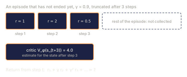
A timeline with rewards 1.0, 2.0 and 0.5 collected in three steps, a dashed block for the rest of the episode that was not collected, a critic box showing V(s_(t+3)) = 4.0 for the state after step 3, and the unfinished return sum with gamma 0.9.
Numbers are illustrative.
8. What is the key difference between the MC advantage and the TD advantage?Explain
A six-step episode with rewards 0, 0, 1, 0, 0, 2 and critic values per step, and two rows marking which cells each advantage reads: the MC row reads every reward, the TD row reads reward 0 and the values at steps 0 and 1; the numbers give A0 of 0.49 (MC) and 0.12 (TD).
Rewards and values are illustrative; advantages computed here.
9. In GAE, what do the two extreme values of λ correspond to?Explain
Line chart of the GAE weight (gamma times lambda) to the power l on the TD residual l steps ahead, for lambda 0, 0.5, 0.95 and 1.0 with gamma 0.99: the lambda 0 line is 1 at offset 0 and 0 after, lambda 1.0 decays slowly from 1 to 0.61 at offset 50.
Weights computed from the formula in the lesson.
10. In the n-step advantage, which settings of n give pure TD and pure MC?Explain
A strip of 12 episode steps with four windows below it: n=1 covers one step, n=2 two steps and n=5 five steps, each ending in a marker where the critic value is read, and n=infinity covers all 12 steps to the end of the episode with no value read.
Schematic of which rewards each window sums.
11. What terms make up the combined actor-critic loss, and what are the canonical coefficient starting points?Explain
A shared trunk feeding an actor head that outputs probabilities 0.7 and 0.3 and a critic head that outputs V(s), with a list of quantities from the batch (advantage, return target, entropy 0.611) and the total loss L as a question mark for one backward pass.
Entropy computed from the example probabilities.
12. Why does A3C not need a replay buffer?Explain
Four worker boxes, each with its own environment and copy of theta, with arrows down to one shared parameter server box that holds theta.
Schematic of the A3C setup from the lesson.
13. A2C collects T=5 steps from each of N=16 parallel environments per rollout. How many transitions are in the combined batch for one update?Apply
A grid of boxes with 16 columns for environments 1 to 16 and 5 rows for steps 1 to 5, each box one transition, and a question for the number of transitions in the combined batch.
14. Using the n-step advantage with n=2, γ=0.5, r_{t+1}=1, r_{t+2}=2, V(s_{t+2})=4 and V(s_t)=1, what is the advantage?Apply
A three-state chain s_t, s_(t+1), s_(t+2) with V(s_t) = 1.0, reward 1 after the first step, reward 2 after the second step and V(s_(t+2)) = 4.0, gamma 0.5, asking for the 2-step advantage.
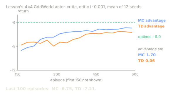
15. Switching from MC to TD advantage cuts the advantage variance sharply, but with a poorly trained critic the policy settles at a worse level than MC reached. Why?Analyze
Learning curves of mean return per episode for an actor-critic on the lesson's GridWorld with a slowly trained critic, the MC advantage curve in blue ending near -6.75 and the TD advantage curve in orange ending near -7.21, with the optimal return of minus 6 dashed, and the mean advantage standard deviation 1.70 for MC and 0.06 for TD.
Real runs of the lesson's code: MC is lam=1 (G minus V), TD is lam=0, critic lr 0.001, actor lr 0.05, 12 seeds, curves averaged over blocks of 25 episodes, first 150 episodes not drawn.
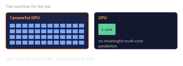
16. You are deploying an actor-critic job on a machine with one powerful GPU and no meaningful multi-core CPU parallelism. Should you reach for A2C or A3C?Design
Two hardware panels: one powerful GPU drawn as a grid of 48 parallel lanes, and a CPU with a single core and no meaningful multi-core parallelism, under a line saying the job is to train an actor-critic and choose A2C or A3C.
Schematic of the stem's machine.

Build It

Step 1: a critic

Linear critic V_φ(s) = w · features(s) updated with MSE:

python
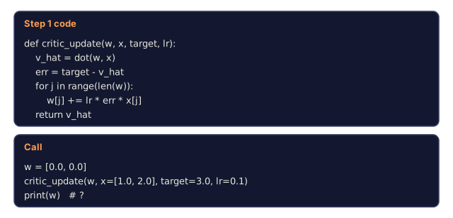
def critic_update(w, x, target, lr):
    v_hat = dot(w, x)
    err = target - v_hat
    for j in range(len(w)):
        w[j] += lr * err * x[j]
    return v_hat

On a tabular env the critic converges in a few hundred episodes. On Atari, replace the linear critic with a shared CNN trunk + value head.

Step 2: n-step advantage

Given a rollout of length T and a bootstrapped final V(s_T):

python
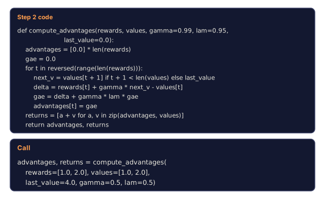
def compute_advantages(rewards, values, gamma=0.99, lam=0.95, last_value=0.0):
    advantages = [0.0] * len(rewards)
    gae = 0.0
    for t in reversed(range(len(rewards))):
        next_v = values[t + 1] if t + 1 < len(values) else last_value
        delta = rewards[t] + gamma * next_v - values[t]
        gae = delta + gamma * lam * gae
        advantages[t] = gae
    returns = [a + v for a, v in zip(advantages, values)]
    return advantages, returns

returns is the critic target. advantages is what multiplies ∇ log π.

Step 3: combined update

python
for step_i, (x, a, _r, probs) in enumerate(traj):
    adv = advantages[step_i]
    target_v = returns[step_i]
 
    # critic
    critic_update(w, x, target_v, lr_v)
 
    # actor
    for i in range(N_ACTIONS):
        grad_logpi = (1.0 if i == a else 0.0) - probs[i]
        for j in range(N_FEAT):
            theta[i][j] += lr_a * adv * grad_logpi * x[j]

On-policy, one rollout per update, separate learning rates for actor and critic.

Step 4: parallelization (A3C vs A2C)

  • A3C: spin up N threads. Each runs its own env and its own forward pass. Periodically push gradient updates to a shared master. No locks on the master: races are fine, they just add noise.
  • A2C: run N env instances in a single process, stack observations into a [N, obs_dim] batch, batched forward pass, batched backward pass. Higher GPU utilization, deterministic, easier to reason about. The default in 2026.

Our toy code is single-threaded for clarity; rewriting to batched A2C is three lines of numpy.
Check: Build It0/5
1. Why is A2C described as easier to reason about than A3C?Explain
Two timelines. For A2C in one process, all environments step together and then one update bar follows, repeated three times at even spacing. For A3C, four worker rows each have their own collecting bars ending in small write markers at different, uneven times.
Schematic with illustrative timings.
2. Calling `critic_update(w, x, target, lr)` with w=[0.0, 0.0], x=[1.0, 2.0], target=3.0, lr=0.1. What is w afterwards?Apply
The critic_update function from Step 1 and a call with w = [0.0, 0.0], x = [1.0, 2.0], target = 3.0, lr = 0.1, followed by print(w) with a question mark for the result.
Code copied from the lesson.
3. `compute_advantages` is called with rewards=[1.0, 2.0], values=[1.0, 2.0], last_value=4.0, gamma=0.5, lam=0.5. What does it return as `returns`?Apply
The compute_advantages function from Step 2 and a call with rewards [1.0, 2.0], values [1.0, 2.0], last_value 4.0, gamma 0.5 and lambda 0.5.
Code copied from the lesson.
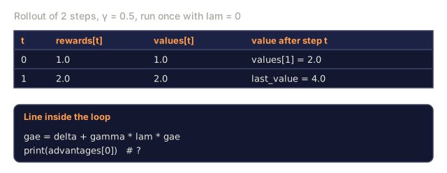
4. The same call (rewards=[1.0, 2.0], values=[1.0, 2.0], last_value=4.0, gamma=0.5) is run with lam=0. What is advantages[0]?Apply
A two-step rollout table (rewards 1.0 and 2.0, values 1.0 and 2.0, last_value 4.0, gamma 0.5) and the line gae = delta + gamma * lam * gae to be run with lam = 0, asking for advantages[0].
Code line copied from the lesson.
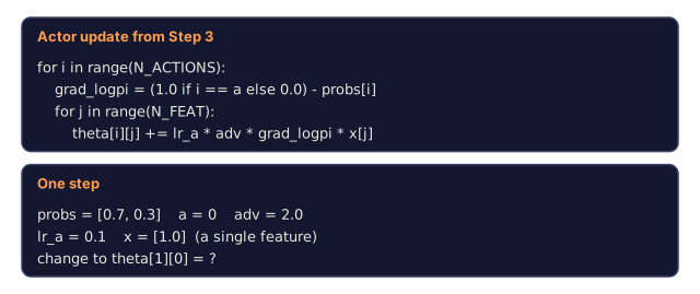
5. In the actor update, one step has probs=[0.7, 0.3], chosen action a=0, adv=2.0, lr_a=0.1 and a single feature x=[1.0]. What is the change to theta[1][0]?Apply
The actor update loop from Step 3 and one step with probs [0.7, 0.3], chosen action 0, adv 2.0, lr_a 0.1 and x = [1.0], asking for the change to theta[1][0].
Code copied from the lesson.

Pitfalls

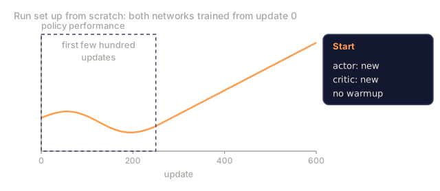
  • Critic bias before actor gradient. If the critic is random, its baseline is uninformative and you're training on pure noise. Warm up the critic for a few hundred steps before turning on the policy gradient, or use a slow actor learning rate.
  • Advantage normalization. Normalize advantages to zero-mean/unit-std per batch. Stabilizes training massively at near-zero cost.
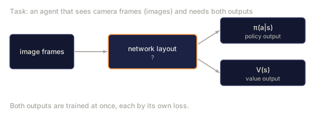
  • Shared trunk. Use a shared feature extractor for actor and critic on image inputs, with separate heads. The shared features free-ride on both losses.
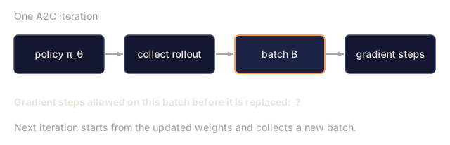
  • On-policy contract. A2C reuses data for exactly one update. Reuse it for more and the gradient turns biased (importance-sampling correction is what PPO adds).
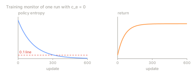
  • Entropy collapse. Without c_e > 0, policy becomes near-deterministic in a few hundred updates and stops exploring.
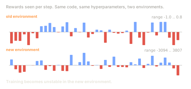
  • Reward scale. Advantage magnitudes depend on reward scale. Normalize rewards (for example, divide by a running standard deviation) for consistent gradient magnitudes across tasks.
Check: Pitfalls0/7
1. What does the lesson mean by A2C's 'on-policy contract,' and what happens if you violate it?Explain
A four-box A2C iteration: policy pi_theta, collect rollout, batch B, gradient steps, followed by the line asking how many gradient steps are allowed on the batch before it is replaced.
Schematic of the lesson's A2C loop.
2. What should you do to advantages before using them in the update, and why?Explain
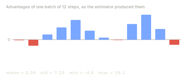
Twelve bars of raw advantages in one batch, positive ones in blue and negative in red, with batch mean 5.59, standard deviation 7.19, minimum -4.6 and maximum 19.1.
Values are illustrative, drawn with numpy.
3. What network layout does the lesson recommend for actor and critic on image inputs?Explain
Image frames going into a box labelled network layout with a question mark, which must produce two outputs: the policy pi(a|s) and the value V(s), each trained by its own loss.
Schematic of the requirement; no layout is shown.
4. You initialize both actor and critic from scratch and start training immediately. For the first few hundred updates, policy performance stays flat or gets worse before it starts climbing. What is the most likely explanation?Analyze
A schematic learning curve of policy performance against update number, flat or slightly declining inside a dashed box labelled first few hundred updates and climbing afterwards, next to a card saying both the actor and the critic are new, with no warmup.
Schematic of the symptom in the question, not measured data.
5. You reuse your actor-critic code on a new environment where rewards run in the thousands instead of roughly [-1, 1], keeping every hyperparameter the same. Training becomes unstable. What should you check first?Analyze
Two rows of per-step reward bars: the old environment with rewards between -1.0 and 0.8, and the new environment with rewards of thousands, from -3094 to 3807, under a line saying training becomes unstable in the new environment.
Rewards are random numbers for illustration.
6. With c_e = 0, a run's policy entropy drops below 0.1 within a few hundred updates and returns stop improving. What is the diagnosis?Analyze
Two small schematic charts for a run with c_e equal to 0: policy entropy against update falls below a dashed line at 0.1 within a few hundred updates, and the return curve against update flattens out.
Schematic of the symptom in the question, not measured data.
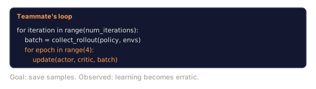
7. A teammate runs four gradient epochs on every A2C rollout to save samples, and learning becomes erratic. Which ingredient is missing?Analyze
A teammate's training loop in which every collected rollout batch is passed through four epochs of update(actor, critic, batch), with the note that the goal is to save samples and learning becomes erratic.
Typed, illustrative code.

Use It

A2C and A3C are rarely the final choice in 2026, but they're the architecture everything later refines:

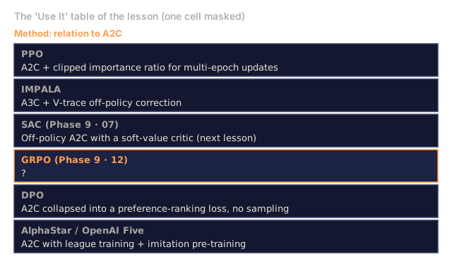
MethodRelation to A2C
PPOA2C + clipped importance ratio for multi-epoch updates
IMPALAA3C + V-trace off-policy correction
SAC (Phase 9 · 07)Off-policy A2C with a soft-value critic (next lesson)
GRPO (Phase 9 · 12)A2C without the critic, group-relative advantage instead
DPOA2C collapsed into a preference-ranking loss, no sampling
AlphaStar / OpenAI FiveA2C with league training + imitation pre-training

If you see "advantage" in a 2026 paper, think actor-critic.
Check: Use It0/2
1. How does the Use It table describe GRPO's relation to A2C?Explain
The lesson's Use It table with columns Method and Relation to A2C: PPO, IMPALA, SAC, DPO and AlphaStar / OpenAI Five have their relation text, and the relation cell of the GRPO row, highlighted, is a question mark.
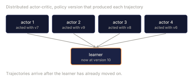
2. You scale a distributed actor-critic with many asynchronous actors, and their policies lag behind the learner so the data is slightly off-policy. Which design fits the lesson's lineage?Design
Four actor boxes that generated data with policy versions 7, 9, 8 and 6, all sending trajectories to a learner box now at version 10.
Version numbers are illustrative.

Ship It

Save as outputs/skill-actor-critic-trainer.md:

markdown
---
name: actor-critic-trainer
description: Produce an A2C / A3C / GAE configuration for a given environment, with advantage estimation and loss weights specified.
version: 1.0.0
phase: 9
lesson: 7
tags: [rl, actor-critic, gae]
---
 
Given an environment and compute budget, output:
 
1. Parallelism. A2C (GPU batched) vs A3C (CPU async) and the number of workers.
2. Rollout length T. Steps per env per update.
3. Advantage estimator. n-step or GAE(λ); specify λ.
4. Loss weights. `c_v` (value), `c_e` (entropy), gradient clip.
5. Learning rates. Actor and critic (separate if using).
 
Refuse single-worker A2C on environments with horizon > 1000 (too on-policy, too slow). Refuse to ship without advantage normalization. Flag any run with `c_e = 0` and observed entropy < 0.1 as entropy-collapsed.
Check: Ship It0/1
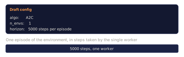
1. An environment has a horizon of 5000 steps and your draft config runs a single-worker A2C. Which change fits the lesson's guidance?Design
A draft config card with algo A2C, n_envs 1 and a horizon of 5000 steps per episode, above one bar for a full episode of 5000 steps played by one worker.
Schematic of the stem's config.

Exercises

  1. Easy. Train actor-critic with MC advantage (G_t - V(s_t)) on 4×4 GridWorld. Compare sample efficiency to REINFORCE-with-running-mean-baseline from Lesson 06.
  2. Medium. Switch to TD-residual advantage (r + γ V(s') - V(s)). Measure variance of the advantage batches. By how much does it drop?
  3. Hard. Implement GAE(λ). Sweep λ ∈ {0, 0.5, 0.9, 0.95, 1.0}. Plot final return vs sample efficiency. Where is the bias/variance sweet spot for this task?

Key Terms

TermWhat people sayWhat it actually means
Actor"The policy net"π_θ(a|s), updated by policy gradient.
Critic"The value net"V_φ(s), updated by MSE regression to returns / TD targets.
Advantage"How much better than average"A(s, a) = Q(s, a) - V(s) or its estimators. Multiplier for ∇ log π.
TD residual"δ"δ_t = r + γ V(s') - V(s); one-step advantage estimate.
GAE"The interpolation knob"Exponentially weighted sum of n-step advantages, parameterized by λ.
A2C"Synchronous actor-critic"Batched across envs; one gradient step per rollout.
A3C"Async actor-critic"Worker threads push gradients to a shared param server. Original paper; less common in 2026.
Bootstrap"Use V at the horizon"Truncate the rollout, add γ^n V(s_{t+n}) to close the sum.

Further Reading

Code

Ships With