TAI BUI
Back to curriculum
BuildPython

Policy Gradient — REINFORCE from Scratch

Stop estimating value. Parameterize the policy directly, compute the gradient of expected return, and step uphill. Williams wrote the whole idea into one theorem in 1992. It's why PPO, GRPO, and every LLM RL loop exist.

TIME: ~75 minutesPREREQUISITES: Phase 3 · 03 (Backpropagation), Phase 9 · 03 (Monte Carlo), Phase 9 · 04 (TD Learning)

Learning Objectives

  • Explain the policy gradient theorem and how the log-derivative trick makes `∇J(θ) = E[G · ∇_θ log π_θ(a|s)]` computable.
  • Implement REINFORCE from scratch (softmax policy, action sampling, episode rollout, and the parameter update) using the closed-form gradient `∇log π(a|s) = e_a - π(·|s)`.
  • Apply baseline subtraction and reward-to-go to cut REINFORCE's variance, and explain why a state-only baseline keeps the gradient estimator unbiased.
  • Place REINFORCE's gradient formula inside PPO, GRPO, DPO, and actor-critic, and diagnose entropy collapse and sample inefficiency in a policy-gradient training run.

The Problem

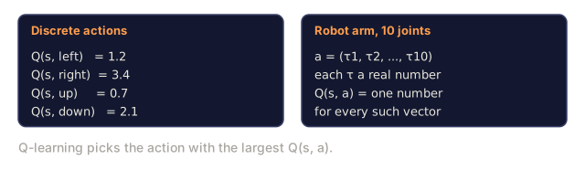
Q-learning and DQN parameterize the value function. You pick actions by argmax Q. That's fine when actions and states are discrete. It breaks once actions go continuous (try taking argmax over a 10-dimensional torque) or once you want a stochastic policy, since argmax is deterministic by construction.

Policy gradients parameterize the policy instead. π_θ(a | s) is a neural net that outputs a distribution over actions. Sample from it to act, compute the gradient of expected return with respect to θ, and step uphill. No argmax, no Bellman recursion. Just gradient ascent on J(θ) = E_{π_θ}[G].

The REINFORCE theorem (Williams 1992) says this gradient is computable: ∇J(θ) = E_π[ G · ∇_θ log π_θ(a | s) ]. Run an episode, compute the return, multiply by ∇ log π_θ(a | s) at every step, average, and take a gradient-ascent step. Done.

Every LLM-RL algorithm running in 2026 (PPO, DPO, GRPO) is a refinement of REINFORCE. Get this one in your fingers and the rest of this phase follows, along with Phase 10 · 07 (RLHF implementation) and Phase 10 · 08 (DPO).
Warm-up0/3
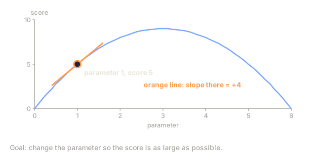
1. You want to make a score as large as possible by adjusting a parameter. Which way should each update move the parameter relative to the score's gradient?Warm-up
A hill-shaped score curve over one parameter from 0 to 6, with a point at parameter 1 where the score is 5 and an orange tangent line showing a slope of +4 there.
Illustrative score curve.
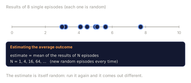
2. You estimate an average outcome by running many random episodes and averaging their results. How does the noise in that estimate change as you average more episodes?Warm-up
A number line from 0 to 10 with the results of eight single random episodes as dots, above a card saying the estimate is the mean of N episodes with N taking the values 1, 4, 16 and 64.
Illustrative episode results.
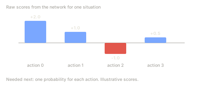
3. A network outputs one raw score per action and you need a probability distribution over the actions. Which function turns the scores into non-negative values that sum to 1?Warm-up
Four bars for the raw scores of actions 0 to 3: +2.0, +1.0, -1.0 and +0.5, one negative, with a note that one probability per action is needed next.
Check: The Problem0/1
1. Why does the lesson say Q-learning-style methods break down for continuous action spaces?Explain
Two panels: a discrete case listing Q values for left, right, up and down, and a robot arm with 10 joints whose action is a vector of ten real-number torques with one Q value per vector, plus the rule that Q-learning picks the action with the largest Q.
Illustrative values.

The Concept

Policy gradient: softmax policy, log-π gradient, return-weighted update

The policy gradient theorem. For any policy π_θ parameterized by θ:

∇J(θ) = E_{τ ~ π_θ}[ Σ_{t=0}^{T} G_t · ∇_θ log π_θ(a_t | s_t) ]

where G_t = Σ_{k=t}^{T} γ^{k-t} r_{k+1} is the discounted return from step t. The expectation is over full trajectories τ sampled from π_θ.

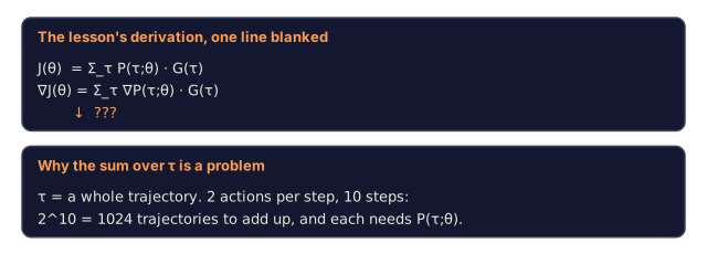
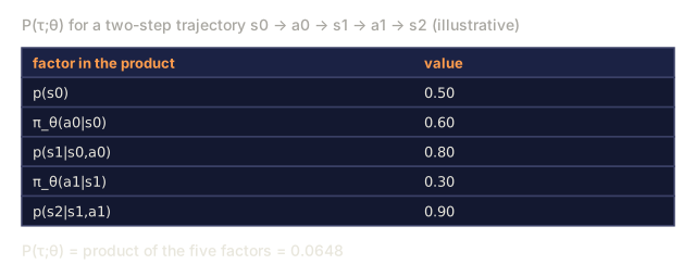
The proof is short. Differentiate J(θ) = Σ_τ P(τ; θ) G(τ) under the expectation. Use ∇P(τ; θ) = P(τ; θ) ∇ log P(τ; θ) (the log-derivative trick). Factor log P(τ; θ) = Σ log π_θ(a_t | s_t) + environment terms that do not depend on θ. The environment terms vanish. Two lines of algebra give you the theorem.

Variance reduction tricks. Vanilla REINFORCE has murderous variance: returns are noisy, ∇ log π is noisy, and their product is even noisier. Two standard fixes:

  1. Baseline subtraction. Replace G_t with G_t - b(s_t) for any baseline b(s_t) that does not depend on a_t. Unbiased because E[b(s_t) · ∇ log π(a_t | s_t)] = 0. Typical choice: b(s_t) = V̂(s_t) learned by a critic → actor-critic (Lesson 07).
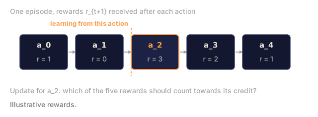
  2. Reward-to-go. Replace Σ_t G_t · ∇ log π_θ(a_t | s_t) with Σ_t G_t^{from t} · ∇ log π_θ(a_t | s_t). Only future returns matter for a given action, since past rewards contribute zero-mean noise.

Combined, you get:

∇J ≈ (1/N) Σ_{i=1}^{N} Σ_{t=0}^{T_i} [ G_t^{(i)} - V̂(s_t^{(i)}) ] · ∇_θ log π_θ(a_t^{(i)} | s_t^{(i)})

which is REINFORCE with a baseline, the direct ancestor of A2C (Lesson 07) and PPO (Lesson 08).

Softmax policy parameterization. For discrete actions, the standard choice:

π_θ(a | s) = exp(f_θ(s, a)) / Σ_{a'} exp(f_θ(s, a'))

where f_θ is any neural net that outputs a score per action. The gradient has a clean form:

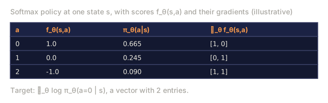
∇_θ log π_θ(a | s) = ∇_θ f_θ(s, a) - Σ_{a'} π_θ(a' | s) ∇_θ f_θ(s, a')

i.e., score of the taken action minus its expected value under the policy.

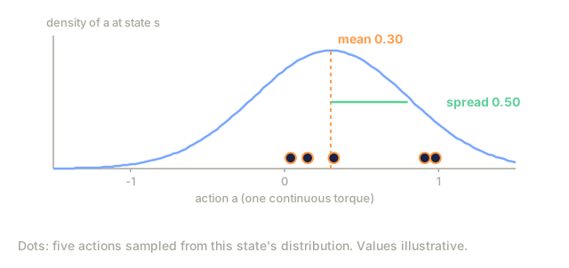
Gaussian policy for continuous actions. π_θ(a | s) = N(μ_θ(s), σ_θ(s)). ∇ log N(a; μ, σ) has a closed form. That is all Phase 9 · 07's SAC needs.
Check: The Concept0/14
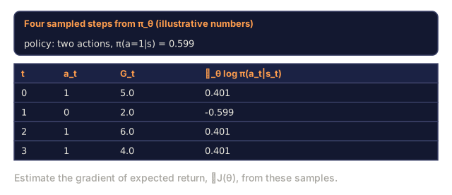
1. What does the REINFORCE theorem say the policy gradient equals?Define
A table of four sampled steps of a two-action policy with action probability 0.599 for action 1: the action taken, the return G and the gradient of the log policy for each step, above a request to estimate the gradient of expected return.
Illustrative numbers.
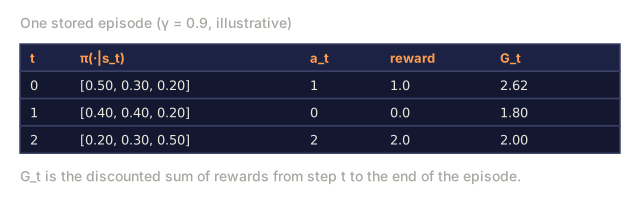
2. What is REINFORCE?Define
A table of one three-step episode with discount 0.9: the action probabilities at each step, the action taken (1, 0, 2), rewards 1.0, 0.0, 2.0 and the returns G_t 2.62, 1.80, 2.00.
Illustrative numbers.
3. What is the 'log-derivative trick' the lesson uses to derive the policy gradient theorem?Define
The first lines of the policy-gradient derivation: J as a sum over trajectories of P times G, then the gradient moved inside the sum, then a blanked step, plus a note that 2 actions for 10 steps give 1024 trajectories.
Illustrative trajectory count.
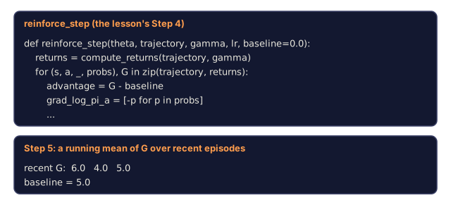
4. What is a baseline in REINFORCE?Define
The reinforce_step code with a baseline=0.0 parameter and the line advantage = G - baseline, and a card showing recent returns 6.0, 4.0, 5.0 with a running-mean baseline of 5.0.
5. What is 'reward-to-go' and why does the lesson say it helps?Define
A row of five steps a_0 to a_4 with rewards 1, 0, 3, 2, 1 and step a_2 outlined, with the question of which rewards should count for the update of a_2.
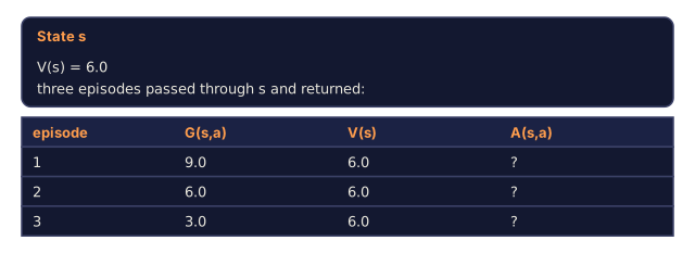
6. What does the advantage A(s, a) = G(s, a) - V(s) measure?Define
A state s with V(s) = 6.0 and three episodes from it returning 9.0, 6.0 and 3.0, in a table with the advantage column A(s,a) blank.
Illustrative numbers.
7. For a softmax policy, what is the closed form the lesson gives for ∇_θ log π_θ(a|s)?Define
A three-action softmax policy at one state: scores 1.0, 0.0, -1.0, the resulting probabilities and a 2-entry score gradient for each action, with the log-policy gradient for action 0 to be found.
Illustrative numbers.
8. How does the lesson define a Gaussian policy for continuous actions?Define
A bell-shaped density curve over one continuous action between -1.5 and 1.5, centered at a mean of 0.30 with a spread of 0.50, with five sampled actions drawn as dots along the axis.
9. Why do the environment's transition probabilities drop out when the policy gradient is derived?Explain
A table of the five factors of the probability of a two-step trajectory: initial state 0.5, policy terms 0.6 and 0.3, and transition terms 0.8 and 0.9, with product 0.0648.
Illustrative numbers.
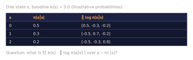
10. Why is subtracting a baseline b(s_t) from the return G_t unbiased, per the lesson?Explain
A state with baseline 3.0 and a table of three actions with probabilities 0.5, 0.3, 0.2 and the log-policy gradient vector for each, asking for the expectation of the baseline times that gradient.
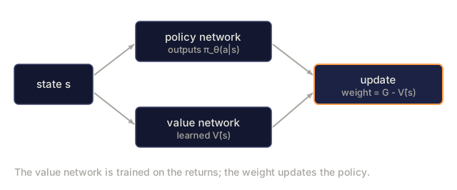
11. How does using a learned value estimate V̂(s) as the baseline change plain REINFORCE?Explain
A diagram: state s feeds a policy network outputting pi and a learned value network outputting V-hat of s, and both feed an update whose weight is G minus V-hat of s.
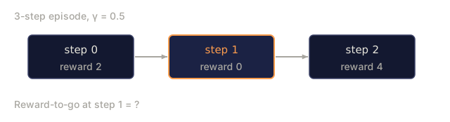
12. A 3-step episode gives rewards 2, 0, 4 at steps 0, 1, 2, and γ = 0.5. What is the reward-to-go at step 1 (that step's reward plus the discounted later rewards)?Apply
Three steps of an episode with rewards 2, 0 and 4 and discount 0.5, step 1 outlined, and the reward-to-go at step 1 left as a question.
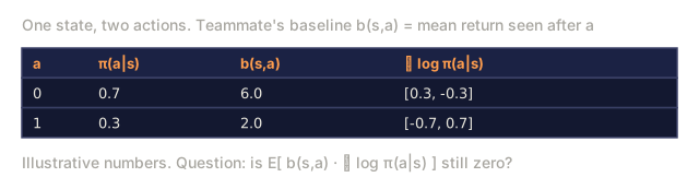
13. A teammate computes the baseline from the action just sampled, b(s_t, a_t), such as the average return seen after that specific action. What goes wrong?Analyze
A state with two actions of probability 0.7 and 0.3, a baseline that depends on the action (6.0 and 2.0) and the log-policy gradient vectors, with the question of whether the expectation of baseline times gradient is still zero.
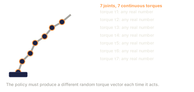
14. You must train a robot arm with 7 continuous joint torques and want a stochastic policy. Which policy head fits?Design
A drawn robot arm with seven joints beside a list of seven torques, each any real number, and a note that the policy must produce a different random torque vector each time it acts.

Build It

Step 1: softmax policy network

python
def policy_logits(theta, state_features):
    return [dot(theta[a], state_features) for a in range(N_ACTIONS)]
 
def softmax(logits):
    m = max(logits)
    exps = [exp(l - m) for l in logits]
    Z = sum(exps)
    return [e / Z for e in exps]

A linear policy works fine here: one weight vector per action, plugged straight into a tabular env. Swap in a CNN and keep the softmax head once you move to Atari.

Step 2: sampling and log-probability

python
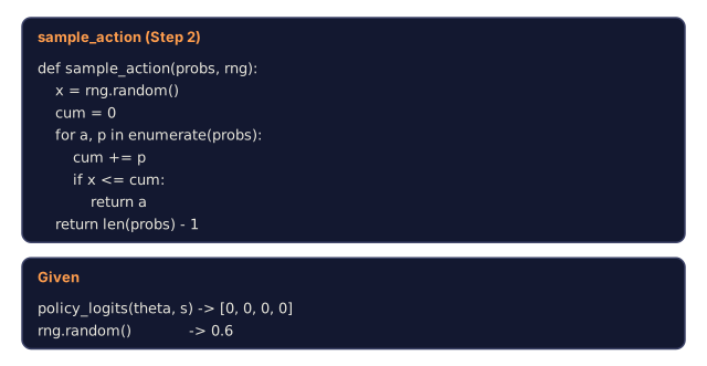
def sample_action(probs, rng):
    x = rng.random()
    cum = 0
    for a, p in enumerate(probs):
        cum += p
        if x <= cum:
            return a
    return len(probs) - 1
 
def log_prob(probs, a):
    return log(probs[a] + 1e-12)

Step 3: rollout with log-probs captured

python
def rollout(theta, env, rng, gamma):
    trajectory = []
    s = env.reset()
    while not done:
        logits = policy_logits(theta, s)
        probs = softmax(logits)
        a = sample_action(probs, rng)
        s_next, r, done = env.step(s, a)
        trajectory.append((s, a, r, probs))
        s = s_next
    return trajectory

Step 4: REINFORCE update

python
def reinforce_step(theta, trajectory, gamma, lr, baseline=0.0):
    returns = compute_returns(trajectory, gamma)
    for (s, a, _, probs), G in zip(trajectory, returns):
        advantage = G - baseline
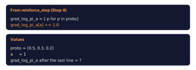
        grad_log_pi_a = [-p for p in probs]
        grad_log_pi_a[a] += 1.0
        for i in range(N_ACTIONS):
            for j in range(len(s)):
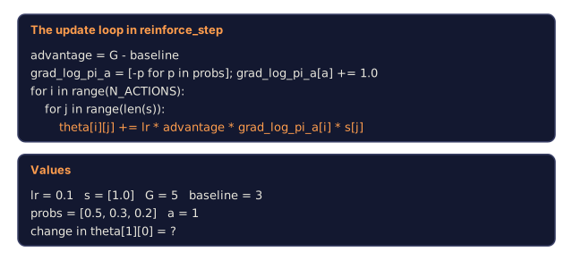
                theta[i][j] += lr * advantage * grad_log_pi_a[i] * s[j]

The gradient ∇ log π(a|s) = e_a - π(·|s), one-hot of a minus the probability vector, is the heart of softmax policy gradients. Burn it into muscle memory.

Step 5: baselines

A running mean of G over recent episodes is enough variance reduction to get a 4×4 GridWorld training, and convergence takes about 500 episodes. Upgrade that baseline to a learned V̂(s) and you've built actor-critic.
Check: Build It0/7
1. With theta set so that policy_logits returns [0, 0, 0, 0], and rng.random() returning 0.6, which action does sample_action return?Apply
The sample_action function from Step 2 with cumulative-sum logic, and the given inputs: all four logits are 0 and rng.random() returns 0.6.
2. A softmax policy gives probs = [0.5, 0.3, 0.2] and the sampled action is a = 1. What does grad_log_pi_a hold in reinforce_step after the line grad_log_pi_a[a] += 1.0?Apply
Two lines from reinforce_step, building grad_log_pi_a from negated probabilities and adding 1.0 at index a, with probs [0.5, 0.3, 0.2], a = 1 and the final list left as a question.
3. In reinforce_step, lr = 0.1, the state is s = [1.0], the return is G = 5, the baseline is 3, probs = [0.5, 0.3, 0.2], and the sampled action is a = 1. By how much does theta[1][0] change?Apply
The double loop of reinforce_step with its update line theta[i][j] += lr * advantage * grad_log_pi_a[i] * s[j] highlighted, and the values lr 0.1, s [1.0], G 5, baseline 3, probs [0.5, 0.3, 0.2], a 1, with the change in theta[1][0] left as a question.
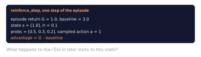
4. In reinforce_step, an episode's return is G = 1.0 and the baseline is 3.0. What happens to the probability of the actions taken in that episode?Apply
Values for one step of reinforce_step: return 1.0, baseline 3.0, state [1.0], learning rate 0.1, probabilities [0.5, 0.3, 0.2] and sampled action 1, with the line advantage = G - baseline.
Illustrative probabilities and learning rate.
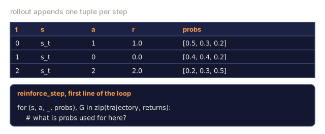
5. In rollout, each step appends (s, a, r, probs). What is probs used for later in reinforce_step?Apply
Three stored rollout tuples (step, state, action, reward, probs) and the first line of the reinforce_step loop that unpacks them, with a comment asking what probs is used for.
Illustrative values.
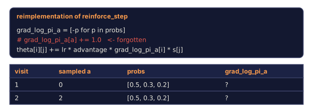
6. A reimplementation builds grad_log_pi_a = [-p for p in probs] but forgets grad_log_pi_a[a] += 1.0. What goes wrong?Analyze
The reinforce_step gradient line with the line adding 1.0 at the sampled action commented out, and two visits to a state with sampled actions 0 and 2 and the same probs [0.5, 0.3, 0.2], with the resulting grad_log_pi_a left as a question.
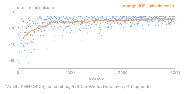
7. Vanilla REINFORCE on a 4x4 GridWorld keeps burning thousands of episodes and its returns swing wildly. What is the cheapest first change the lesson recommends?Analyze
A scatter of the returns of 3000 episodes of vanilla REINFORCE without a baseline on a 4x4 GridWorld, with a 100-episode moving average. Individual returns range from about -63 to -6, widest in the first few hundred episodes; the average climbs slowly from about -33 to -9 and individual returns still scatter by several points at the end.
Real run of the lesson's main.py code with use_baseline=False, a small learning rate of 0.0005 (the file uses 0.05), seed 0, gamma 0.99. Returns are G_0.

Pitfalls

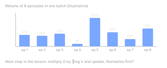
  • Exploding gradients. Returns can be huge. Always normalize G to ~N(0, 1) across the batch before multiplying by ∇ log π.
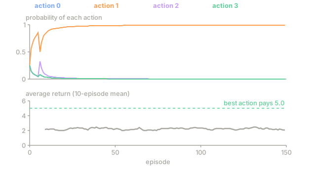
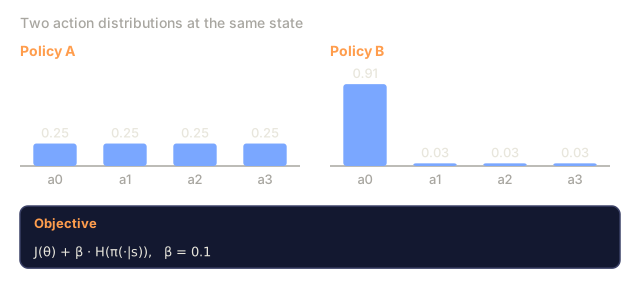
  • Entropy collapse. The policy converges on a near-deterministic action too early, stops exploring, and gets stuck. Fix: add an entropy bonus β · H(π(·|s)) to the objective.
  • High variance. Vanilla REINFORCE needs thousands of episodes to converge. A critic baseline (Lesson 07) or TRPO/PPO's trust region (Lesson 08) is the standard fix.
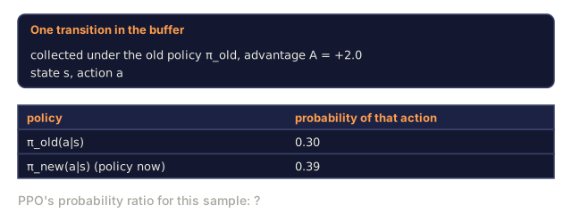
  • Sample inefficiency. On-policy means every transition gets thrown away after one update. Off-policy corrections via importance sampling bring old data back, at the cost of variance: PPO's ratio is exactly a clipped IS weight.
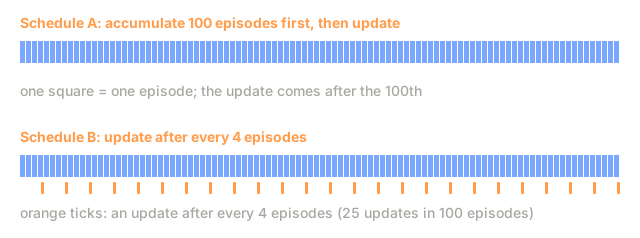
  • Non-stationary gradients. A gradient computed from episodes 100 steps old is using a stale π. That's why on-policy methods update every few rollouts instead of hoarding data.
  • Credit assignment. Skip reward-to-go and past rewards just add noise to the credit signal. Always use reward-to-go.
Check: Pitfalls0/9
1. What does an entropy bonus β · H(π(·|s)) do when added to the objective?Define
Bars for two action distributions over four actions: policy A with 0.25 each and policy B with 0.91, 0.03, 0.03, 0.03, above the objective J(θ) plus beta times the entropy of the policy with beta = 0.1.
Illustrative probabilities.
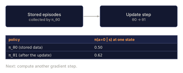
2. What does it mean that policy-gradient training is on-policy?Define
A box of stored episodes collected by the old policy, an update step from theta 0 to theta 1, and a table of the probability of action 0 at one state: 0.50 under the old policy and 0.62 under the updated one.
Illustrative numbers.
3. Why does the lesson say to normalize G to roughly zero mean and unit variance across the batch before multiplying by ∇log π?Explain
Eight bars for the returns of the episodes in one batch, ranging from 90 to 1020, with a note that the next step multiplies G by the log-policy gradient.
4. Why does the lesson say on-policy methods must update every few rollouts rather than accumulating many episodes first?Explain
Two rows of 100 episode squares: schedule A has a single update after the 100th episode, schedule B has an update after every 4 episodes, 25 updates in total.
Illustrative schedules.
5. What is PPO's probability ratio, given the lesson's discussion of sample inefficiency?Explain
One stored transition collected under the old policy with advantage +2.0, and a table of the probability of its action: 0.30 under the old policy and 0.39 under the current one, with PPO's ratio for it left as a question.
Illustrative numbers.
6. During training, your policy's action probabilities collapse toward a single action within the first few dozen episodes, and the average return plateaus well below what looks achievable. What's happening, and what's the standard fix?Analyze
Two plots of one training run on a four-action task: the probability of each action over 150 episodes, where one action reaches a probability near 1 within the first few dozen episodes, and the 10-episode average return, which stays between about 2 and 2.5 while the best action pays 5.0.
Real numpy REINFORCE run on a toy 4-action task (action means 2.0, 2.2, 2.4, 5.0), seed 19. Illustrative.
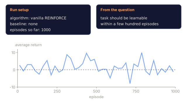
7. You train vanilla REINFORCE with no baseline on a task that should be learnable within a few hundred episodes. After a thousand episodes, the return is still bouncing around with no clear upward trend. What's the most likely explanation?Analyze
A run-setup card for vanilla REINFORCE with no baseline after 1000 episodes, a card saying the task should be learnable in a few hundred, and a learning curve of 25-episode average returns that jumps between about -8 and +10 with no steady rise.
Real run, not a schematic: vanilla REINFORCE on a toy 4-action task (action means 2.0, 2.2, 2.4, 5.0, reward noise std 20), lr 0.002, seed 2. Each point is the mean return of 25 episodes. Stands in for the question's task.
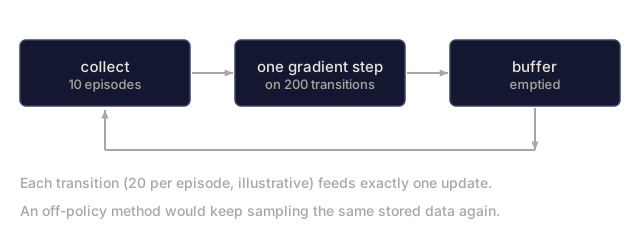
8. Your on-policy REINFORCE agent throws away every transition right after one gradient update, so it needs far more environment interaction than an off-policy method would. What's the standard partial fix, and what does it cost?Analyze
A loop of three boxes: collect 10 episodes, one gradient step on 200 transitions, buffer emptied, with an arrow back to collect, and notes that each transition is used by exactly one update.
Illustrative sizes: 10 episodes of 20 transitions each.
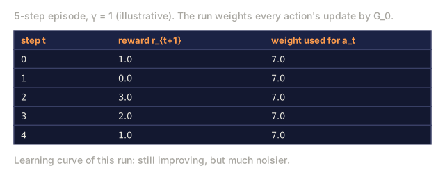
9. A run uses the full return G_0 for every step's update instead of reward-to-go. It still learns, but the learning curve is much noisier. Why?Analyze
A five-step episode with rewards 1, 0, 3, 2, 1 and discount 1, where every step's update uses the same weight G_0 = 7.0, and a note that the learning curve still improves but is much noisier.

Use It

By 2026, REINFORCE is rarely run directly, but its gradient formula is everywhere you look:

Use caseDerived method
Continuous controlPPO / SAC with Gaussian policy
LLM RLHFPPO with KL penalty, running on token-level policy
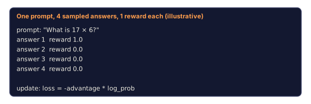
LLM reasoning (DeepSeek)GRPO: REINFORCE with group-relative baseline, no critic
Multi-agentCentralized-critic REINFORCE (MADDPG, COMA)
Discrete action roboticsA2C, A3C, PPO
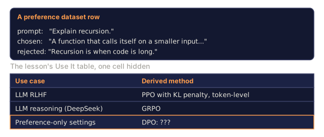
Preference-only settingsDPO: REINFORCE rewritten as a preference-likelihood loss, no sampling

When you spot loss = -advantage * log_prob in a 2026 training script, that line is REINFORCE with a baseline. Whole papers, DPO, GRPO, and RLOO among them, amount to variance-reduction tricks stacked on top of it.
Check: Use It0/3
1. How does the lesson describe GRPO's relationship to REINFORCE?Explain
A prompt with four sampled answers and rewards 1.0, 0.0, 0.0, 0.0, and the update line loss = -advantage * log_prob.
2. How does the Use It table describe DPO's relationship to REINFORCE?Explain
A preference dataset row with a prompt, a chosen answer and a rejected answer, above three rows of the Use It table (RLHF, reasoning, preference-only settings) with the DPO entry blanked.
Dataset row is illustrative; table cells are shortened from the lesson.
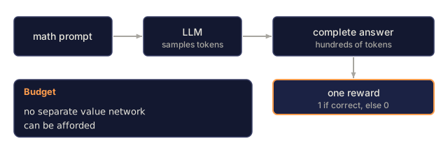
3. You fine-tune an LLM on math problems with one reward per complete answer and cannot afford a separate value network. Which design fits the lesson's ideas?Design
A pipeline: a math prompt goes into an LLM that samples a complete answer of hundreds of tokens, which receives one reward, 1 if correct and 0 otherwise, beside a note that no separate value network can be afforded.
Token count and the 0/1 reward values are illustrative.

Ship It

Save as outputs/skill-policy-gradient-trainer.md:

markdown
---
name: policy-gradient-trainer
description: Produce a REINFORCE / actor-critic / PPO training config for a given task and diagnose variance issues.
version: 1.0.0
phase: 9
lesson: 6
tags: [rl, policy-gradient, reinforce]
---
 
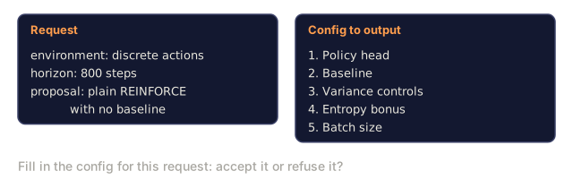
Given an environment (discrete / continuous actions, horizon, reward stats), output:
 
1. Policy head. Softmax (discrete) or Gaussian (continuous) with parameter counts.
2. Baseline. None (vanilla), running mean, learned `V̂(s)`, or A2C critic.
3. Variance controls. Reward-to-go on by default, return normalization, gradient clip value.
4. Entropy bonus. Coefficient β and decay schedule.
5. Batch size. Episodes per update; on-policy data freshness contract.
 
Refuse REINFORCE-no-baseline on horizons > 500 steps. Refuse continuous-action control with a softmax head. Flag any run with `β = 0` and observed policy entropy < 0.1 as entropy-collapsed.
Check: Ship It0/1
1. A task has a horizon of 800 steps and a colleague proposes plain REINFORCE with no baseline. What should the trainer config do?Design
A request card with discrete actions, a horizon of 800 steps and a plain REINFORCE proposal with no baseline, beside the five config items from the policy-gradient-trainer skill: policy head, baseline, variance controls, entropy bonus and batch size.
Author's Note

When I first implemented REINFORCE, I skipped baseline subtraction and reward-to-go because they read like footnotes to the theorem. They aren't. Vanilla REINFORCE on anything harder than a 4x4 grid burns thousands of episodes fighting its own variance, and you'll spend that time convinced your code is broken when the algorithm is just doing what vanilla REINFORCE does. Add the running-mean baseline first: it's three lines of code and the most effective change you can make before reaching for a critic network.

The other thing worth saying out loud: once you've written advantage * log_prob by hand, GRPO and DPO stop looking like new algorithms. They're REINFORCE with a different baseline and a different way of dodging on-policy sampling. Spotting that pattern is worth more than memorizing any one paper's notation.

Exercises

  1. Easy. Implement REINFORCE on 4×4 GridWorld with a linear softmax policy. Train for 1,000 episodes without a baseline. Plot the learning curve; measure variance (std of returns).
  2. Medium. Add a running-mean baseline. Train again. Compare sample efficiency and variance to the vanilla run. By how much does the baseline reduce steps to convergence?
  3. Hard. Add an entropy bonus β · H(π). Sweep β ∈ {0, 0.01, 0.1, 1.0}. Plot final return and policy entropy. Where is the sweet spot on this task?

Key Terms

TermWhat people sayWhat it actually means
Policy gradient"Train the policy directly"∇J(θ) = E[G · ∇ log π_θ(a|s)]; derived from the log-derivative trick.
REINFORCE"The original PG algorithm"Williams (1992); Monte Carlo returns multiplied by log-policy gradient.
Log-derivative trick"Score function estimator"∇P(τ;θ) = P(τ;θ) · ∇ log P(τ;θ); makes gradients of expectations tractable.
Baseline"Variance reduction"Any b(s) subtracted from G; unbiased because E[b · ∇ log π] = 0.
Reward-to-go"Only future returns count"G_t^{from t} instead of the full G_0; correct and lower-variance.
Entropy bonus"Encourage exploration"+β · H(π(·|s)) term keeps the policy from collapsing.
On-policy"Train on what you just saw"Gradient expectation is w.r.t. the current policy, so old data can't be reused directly.
Advantage"How much better than average"A(s, a) = G(s, a) - V(s); the signed quantity REINFORCE-with-baseline multiplies.

Further Reading

Code

Ships With