Deep Q-Networks (DQN)
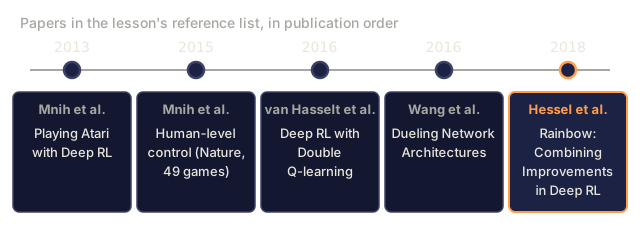
2013: Mnih trained a single Q-learning network on raw pixels and beat every classical RL agent on seven Atari games. 2015: the same idea scaled to 49 games, landed in Nature, and kicked off the deep-RL era. DQN is just Q-learning plus three tricks that make function approximation hold together.
Learning Objectives
- Explain why tabular Q-learning cannot scale past a few thousand states, and how a neural Q-function Q(s, a; θ) replaces the lookup table.
- Name DQN's three stabilization tricks (experience replay, target network, reward clipping) and the deadly-triad failure mode each one counters.
- Implement a full DQN training loop from scratch in stdlib Python: replay buffer, Q-network, ε-greedy action selection, and periodic target-network sync.
- Apply Double DQN's action-selection/evaluation split to fix maximization bias, and place DQN correctly against SAC/TD3, PPO, and offline RL for a given task.
The Problem
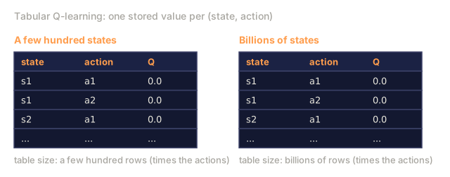
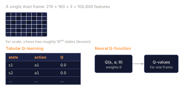
Tabular Q-learning needs a separate Q-value for every (state, action) pair. A chess board has roughly 10⁴³ states. A single Atari frame is 210×160×3 = 100,800 features. Tabular RL dies at thousands of states, let alone billions.
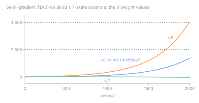
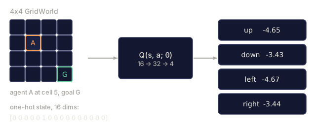
The fix looks obvious in hindsight: swap the Q-table for a neural network, Q(s, a; θ). Obvious in hindsight took decades to actually work, because naive function approximation with Q-learning diverges under the "deadly triad": function approximation plus bootstrapping plus off-policy learning. Mnih et al. (2013, 2015) found three engineering tricks that stabilize the whole thing:
- Experience replay decorrelates transitions.
- Target network freezes the bootstrap target.
- Reward clipping normalizes gradient magnitudes.
DQN on Atari was the first time a single architecture with a single hyperparameter set solved dozens of control problems straight from raw pixels. Everything "deep-RL" built since (DDQN, Rainbow, Dueling, Distributional, R2D2, Agent57) stacks on top of this three-trick base.
The Concept

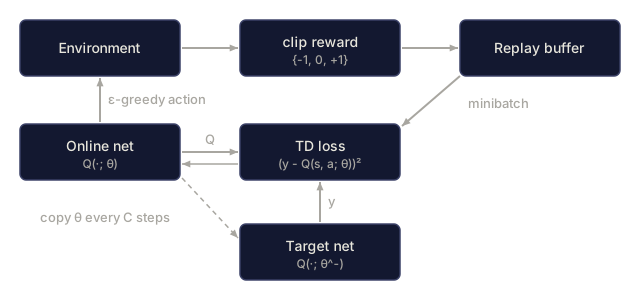
The objective. DQN minimizes the one-step TD loss on a neural Q-function:
L(θ) = E_{(s,a,r,s')~D} [ (r + γ max_{a'} Q(s', a'; θ^-) - Q(s, a; θ))² ]
θ is the online network, updated every step by gradient descent. θ^- is the target network, periodically copied from θ (every ~10,000 steps). D is the replay buffer of past transitions.
The three tricks, in order of importance:
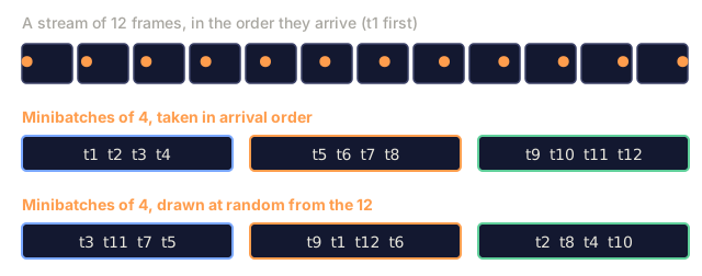
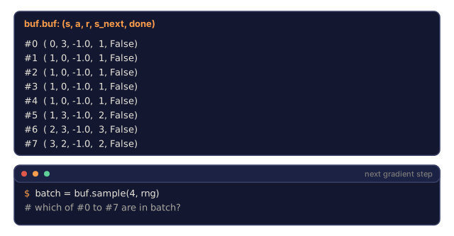
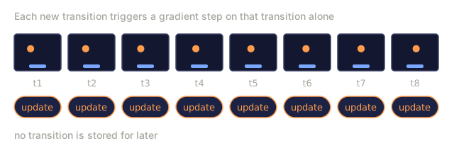
Experience replay. A ring buffer of ~10⁶ transitions. Each training step samples a minibatch uniformly at random. This breaks temporal correlation (successive frames are nearly identical), lets the network learn from rare rewarding transitions many times, and decorrelates consecutive gradient updates. Without it, on-policy TD with a neural net diverges on Atari.
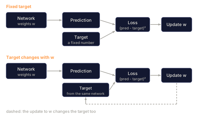
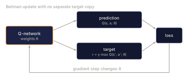
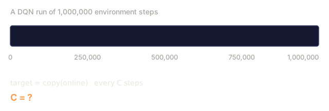
Target network. A second copy of the Q-network, Q(·; θ^-), with its weights frozen and periodically copied from the online network: θ → θ^- every C steps. It exists because using the same network Q(·; θ) on both sides of the Bellman equation makes the target move every update, so the network ends up chasing its own tail. The frozen copy stabilizes the regression target for thousands of gradient steps at a stretch. Soft updates, θ^- ← τ θ + (1-τ) θ^- (used in DDPG, SAC), are a smoother variant.
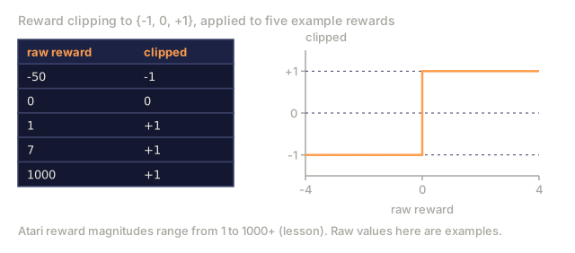
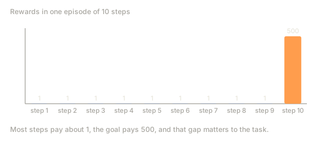
Reward clipping. Clip every reward to {-1, 0, +1}. Atari reward magnitudes vary from 1 to 1000+, so without clipping, one game's scale would dominate the gradient. Wrong when reward magnitude matters; fine for Atari, where only sign matters.
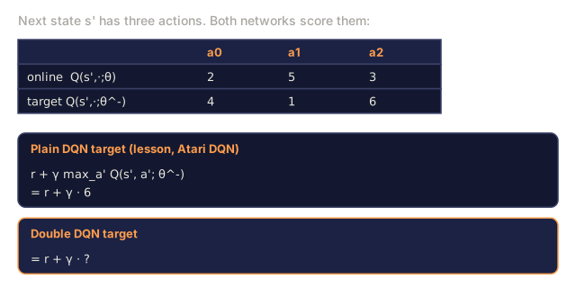
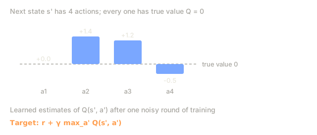
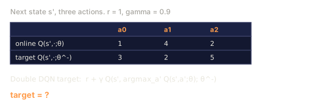
Double DQN. Hasselt (2016) fixes maximization bias: use the online net to select the action, the target net to evaluate it.
target = r + γ Q(s', argmax_{a'} Q(s', a'; θ); θ^-)
Drop-in replacement, consistently better. Use it by default.
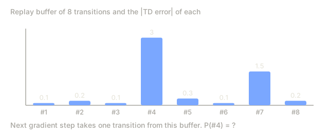
Other improvements (Rainbow, 2017): prioritized replay (sample high-TD-error transitions more), dueling architecture (separate V(s) and advantage heads), noisy networks (learned exploration), n-step returns, distributional Q (C51/QR-DQN), multi-step bootstrapping. Each adds a few percent; the gains are roughly additive.
Build It
The code here is stdlib-only, no NumPy: a hand-rolled single-hidden-layer MLP running on a tiny continuous GridWorld, so every training step takes microseconds. The algorithm is identical to Atari DQN, just at a much smaller scale.
Step 1: replay buffer
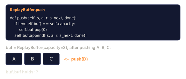
class ReplayBuffer:
    def __init__(self, capacity):
        self.buf = []
        self.capacity = capacity
    def push(self, s, a, r, s_next, done):
        if len(self.buf) == self.capacity:
            self.buf.pop(0)
        self.buf.append((s, a, r, s_next, done))
    def sample(self, batch, rng):
        return rng.sample(self.buf, batch)
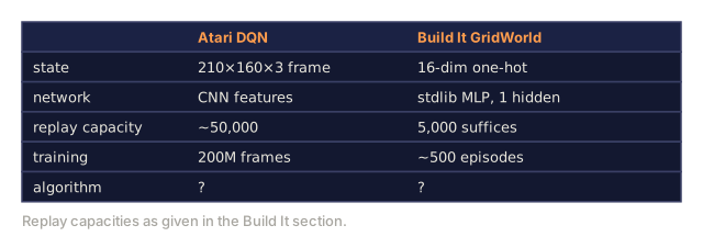
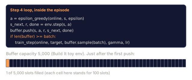
~50,000 capacity for Atari; 5,000 suffices for this toy env.
Step 2: a tiny Q-network (manual MLP)
class QNet:
    def __init__(self, n_in, n_hidden, n_actions, rng):
        self.W1 = [[rng.gauss(0, 0.3) for _ in range(n_in)] for _ in range(n_hidden)]
        self.b1 = [0.0] * n_hidden
        self.W2 = [[rng.gauss(0, 0.3) for _ in range(n_hidden)] for _ in range(n_actions)]
        self.b2 = [0.0] * n_actions
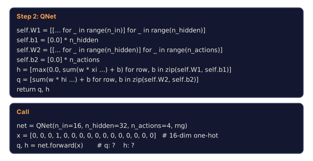
    def forward(self, x):
        h = [max(0.0, sum(w * xi for w, xi in zip(row, x)) + b) for row, b in zip(self.W1, self.b1)]
        q = [sum(w * hi for w, hi in zip(row, h)) + b for row, b in zip(self.W2, self.b2)]
        return q, h
Forward pass: linear → ReLU → linear. That is the entire net.
Step 3: the DQN update
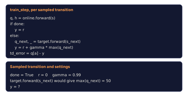
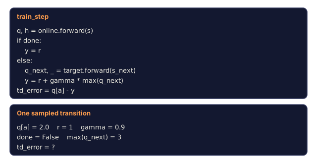
def train_step(online, target, batch, gamma, lr):
    grads = zeros_like(online)
    for s, a, r, s_next, done in batch:
        q, h = online.forward(s)
        if done:
            y = r
        else:
            q_next, _ = target.forward(s_next)
            y = r + gamma * max(q_next)
        td_error = q[a] - y
        accumulate_grads(grads, online, s, h, a, td_error)
    apply_sgd(online, grads, lr / len(batch))
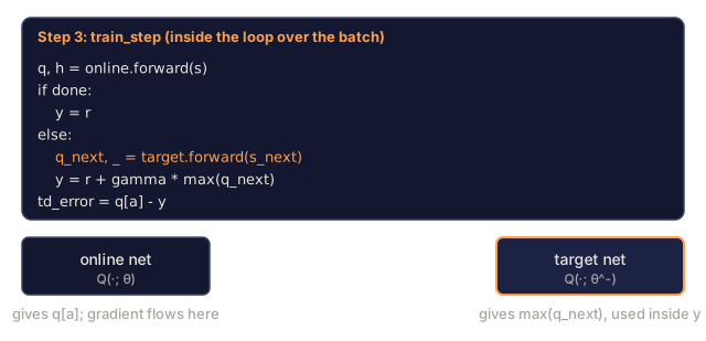
The shape is Q-learning from Lesson 04 with two differences: you backprop through a differentiable Q(·; θ) instead of indexing a table, and the target uses Q(·; θ^-).
Step 4: the outer loop
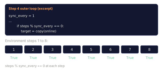
For each episode, act ε-greedy on Q(·; θ), push transitions into the buffer, sample a minibatch, take a gradient step, periodically sync θ^- ← θ. The pattern:
for episode in range(N):
    s = env.reset()
    while not done:
        a = epsilon_greedy(online, s, epsilon)
        s_next, r, done = env.step(s, a)
        buffer.push(s, a, r, s_next, done)
        if len(buffer) >= batch:
            train_step(online, target, buffer.sample(batch), gamma, lr)
        if steps % sync_every == 0:
            target = copy(online)
        s = s_next
On this tiny GridWorld with a 16-dim one-hot state, the agent learns a near-optimal policy in about 500 episodes. On Atari, scale this up to 200M frames and add a CNN feature extractor.
Pitfalls
- Deadly triad. Function approximation + off-policy + bootstrapping can diverge. DQN mitigates with target net + replay; do not remove either.
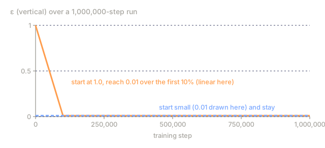
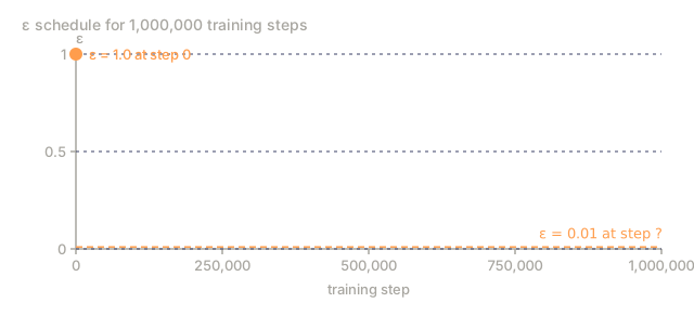
- Exploration. ε must decay, typically from 1.0 to 0.01 over the first ~10% of training. Without enough early exploration the Q-net converges to a local basin.
- Overestimation.
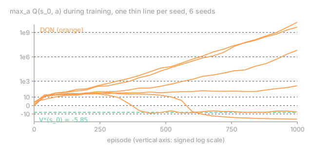
maxover noisy Q is upward-biased. Always use Double DQN in production. - Reward scale. Clip or normalize rewards; the gradient magnitude is proportional to reward magnitude.
- Replay buffer coldstart. Don't train until the buffer has a few thousand transitions. Early gradients on ~20 samples overfit.
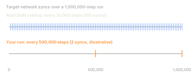
- Target sync frequency. Too frequent ≈ no target net; too infrequent ≈ stale targets. Atari DQN uses 10,000 env steps. Rule of thumb: sync every ~1/100 of training horizon.
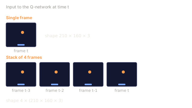
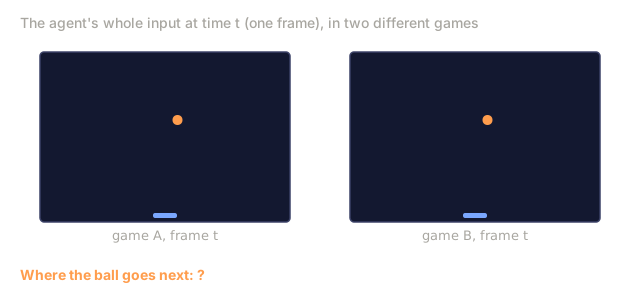
- Observation preprocessing. Atari DQN stacks 4 frames to make state Markov. Any env with velocity info needs frame-stacking or recurrent state.
Use It
In 2026, DQN is rarely state-of-the-art but remains the reference off-policy algorithm:
| Task | Method of choice | Why not DQN? |
|---|---|---|
| Discrete-action Atari-like | Rainbow DQN or Muesli | Same framework, more tricks. |
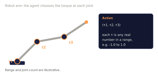
| Continuous control | SAC / TD3 (Phase 9 · 07) | DQN has no policy network. |
| On-policy / high-throughput | PPO (Phase 9 · 08) | No replay buffer; easier to scale. |
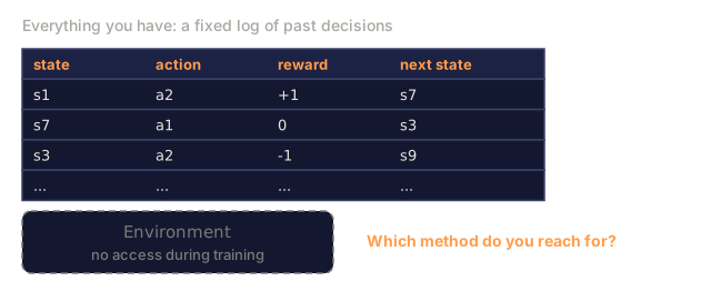
| Offline RL | CQL / IQL / Decision Transformer | Conservative Q targets, no bootstrapping blowups. |
| Large discrete action spaces (recommender) | DQN with action embedding, or IMPALA | Fine; decoration matters. |
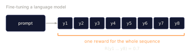
| LLM RL | PPO / GRPO | Sequence-level, not step-level; different loss. |
The lessons still travel. Replay and target networks appear in SAC, TD3, DDPG, SAC-X, AlphaZero's self-play buffer, and every offline RL method. Reward clipping lives on as advantage normalization in PPO. The architecture is the blueprint.
Ship It
Save as outputs/skill-dqn-trainer.md:
---
name: dqn-trainer
description: Produce a DQN training config (buffer, target sync, ε schedule, reward clipping) for a discrete-action RL task.
version: 1.0.0
phase: 9
lesson: 5
tags: [rl, dqn, deep-rl]
---

Given a discrete-action environment (observation shape, action count, horizon, reward scale), output:

1. Network. Architecture (MLP / CNN / Transformer), feature dim, depth.
2. Replay buffer. Capacity, minibatch size, warmup size.
3. Target network. Sync strategy (hard every C steps or soft τ).
4. Exploration. ε start / end / schedule length.
5. Loss. Huber vs MSE, gradient clip value, reward clipping rule.
6. Double DQN. On by default unless explicit reason to disable.

Refuse to ship a DQN with no target network, no replay buffer, or ε held at 1. Refuse continuous-action tasks (route to SAC / TD3). Flag any reward range > 10× per-step mean as needing clipping or scale normalization.
Exercises
- Easy. Run
code/main.py. Plot the per-episode return curve. How many episodes until the running mean exceeds -10? - Medium. Disable the target network (use the online net for both sides of the Bellman target). Measure training instability: does return oscillate or diverge?
- Hard. Add Double DQN: use the online net to pick
argmax a', target net to evaluate. Compare bias ofQ(s_0, best_a)vs trueV*(s_0)after 1,000 episodes with vs without Double DQN on a noisy-reward GridWorld.
Key Terms
| Term | What people say | What it actually means |
|---|---|---|
| DQN | "Deep Q-learning" | Q-learning with a neural Q-function, replay buffer, and target network. |
| Experience replay | "Shuffled transitions" | Ring buffer sampled uniformly each gradient step; decorrelates data. |
| Target network | "Frozen bootstrap" | Periodic copy of Q used in the Bellman target; stabilizes training. |
| Deadly triad | "Why RL diverges" | Function approximation + bootstrapping + off-policy = no convergence guarantee. |
| Double DQN | "Fix for maximization bias" | Online net selects action, target net evaluates it. |
| Dueling DQN | "V and A heads" | Decompose Q = V + A - mean(A); same output, better gradient flow. |
| Rainbow | "All the tricks" | DDQN + PER + dueling + n-step + noisy + distributional in one. |
| PER | "Prioritized Replay" | Sample transitions proportional to TD-error magnitude. |
Further Reading
- Mnih et al. (2013). Playing Atari with Deep Reinforcement Learning: the 2013 NeurIPS workshop paper that kicked off deep RL.
- Mnih et al. (2015). Human-level control through deep reinforcement learning: the Nature paper, 49-game DQN.
- Hasselt, Guez, Silver (2016). Deep Reinforcement Learning with Double Q-learning: DDQN.
- Wang et al. (2016). Dueling Network Architectures: dueling DQN.
- Hessel et al. (2018). Rainbow: Combining Improvements in Deep RL: the stacked-tricks paper.
- OpenAI Spinning Up: DQN: clear modern exposition.
- Sutton & Barto (2018), Ch. 9: On-policy Prediction with Approximation: the textbook treatment of the "deadly triad" (function approximation, bootstrapping, off-policy) that DQN's target network and replay buffer are built to tame.
- CleanRL DQN implementation: reference single-file DQN used in ablation studies, good to read alongside this lesson's from-scratch version.
Code
- main.py (python, 183 lines)