BuildPython

DPO: Direct Preference Optimization

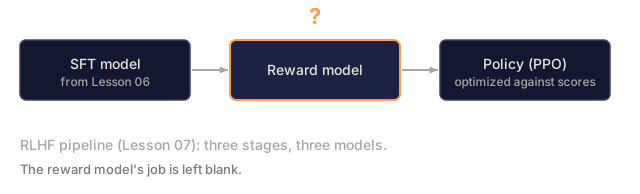
RLHF works, but it takes three models (SFT, reward model, policy), PPO's instability, and a KL penalty you have to tune. DPO asks whether you can skip all of that. It optimizes the language model directly on preference pairs: no reward model, no PPO, one training loop.

TIME: ~90 minutesPREREQUISITES: Phase 10, Lesson 07 (RLHF)

Learning Objectives

Implement DPO training that directly optimizes a language model on preference pairs without a separate reward model
Derive the DPO loss function and explain how it implicitly represents a reward model through the policy's log probabilities
Compare DPO vs RLHF in terms of training stability, compute cost, and number of models required
Tune the beta parameter to control how far the trained policy diverges from the reference model

The Problem

You built an RLHF pipeline in Lesson 07. Three stages. Three models. The SFT model, the reward model, and the policy model optimized with PPO. The reward model alone required thousands of human preference pairs and a separate training loop. PPO required careful tuning of the KL coefficient, learning rate, clip ratio, and number of epochs.

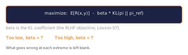
In practice, PPO training is notoriously unstable. Small hyperparameter changes cause the training to diverge. The reward model is an imperfect proxy for human preferences, and the policy finds ways to exploit its weaknesses. The KL penalty helps but requires its own tuning. Too low and you get reward hacking, too high and the model barely learns.

This complexity is why most open-source models struggled with RLHF for years after InstructGPT was published. The three-stage pipeline is fragile. Each stage has its own failure modes, and errors compound.

In May 2023, Rafael Rafailov, Archit Sharma, and colleagues at Stanford published "Direct Preference Optimization: Your Language Model is Secretly a Reward Model." The key insight: you don't need a separate reward model. The optimal reward function is mathematically determined by the language model's own token probabilities. You can skip the reward model entirely and optimize the language model directly on preference pairs.

DPO reduces RLHF to a single supervised learning step. One model. One loss function. One training loop. No reinforcement learning. Zephyr-7B, one of the first models to use DPO at scale, matched or beat models trained with full RLHF on several benchmarks. Meta used DPO as part of Llama 3's alignment pipeline. Anthropic has cited DPO-style methods in their alignment research.

Warm-up0/4

1. In the RLHF pipeline from Lesson 07, what is the reward model's job?Warm-up

The RLHF pipeline from Lesson 07; the reward model's job is the question.

2. What does the KL penalty do in RLHF, and why does it need tuning?Warm-up

The RLHF objective, maximizing expected reward minus beta times a KL penalty, with two blanks asking what happens when beta is too low and too high. — The literal RLHF objective from Lesson 07.

3. A sigmoid function takes any real number as input. What range of outputs does it produce?Warm-up

Five real numbers from -1000 to 1000, each feeding a sigmoid unit, with every output p left as a question mark.

4. For positive numbers a and b, which identity holds for logarithms?Warm-up

Two positive numbers, a = 24 and b = 3, with log(a), log(b) and log(a/b) all left as question marks.

Check: The Problem0/1

1. What is DPO (Direct Preference Optimization)?Define

A real preference-pair example from the lesson's data about explaining gravity, with a short preferred answer and a longer rejected answer. — Real entry from the lesson's PREFERENCE_DATA list.

The Concept

The Key Insight

RLHF optimizes this objective:

maximize: E[R(x, y)] - beta * KL(pi || pi_ref)

where R is the reward model, pi is the policy, pi_ref is the reference model, and beta is the KL coefficient.

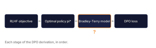
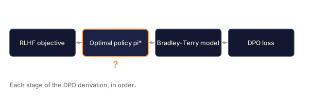
The DPO paper showed that this objective has a closed-form optimal solution. For any reward function R, the optimal policy is:

pi*(y | x) = pi_ref(y | x) * exp(R(x, y) / beta) / Z(x)

where Z(x) is a normalizing constant. Rearranging:

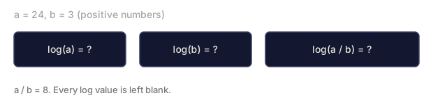
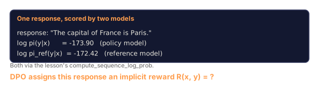
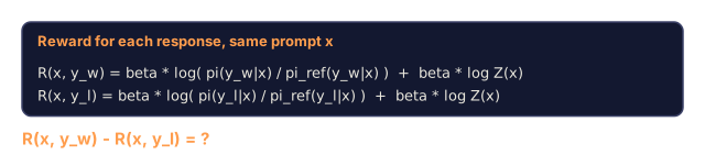
R(x, y) = beta * log(pi*(y | x) / pi_ref(y | x)) + beta * log Z(x)

This is the breakthrough. The reward is expressed entirely in terms of the policy model's probabilities and the reference model's probabilities. You don't need to train a separate reward model. The reward is implicit in the probability ratio.

Substituting this into the Bradley-Terry preference model:

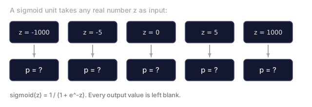
P(y_w > y_l | x) = sigmoid(R(x, y_w) - R(x, y_l))
                  = sigmoid(beta * (log pi(y_w|x)/pi_ref(y_w|x) - log pi(y_l|x)/pi_ref(y_l|x)))

The Z(x) terms cancel because both responses condition on the same prompt x. What's left is a function of only the policy model's log-probabilities and the reference model's log-probabilities on the preferred and rejected responses.

The DPO Loss

L_DPO = -log(sigmoid(beta * (log pi(y_w|x)/pi_ref(y_w|x) - log pi(y_l|x)/pi_ref(y_l|x))))

Let's unpack each piece:

y_w = preferred (winning) response
y_l = rejected (losing) response
x = prompt
pi = current model (being trained)
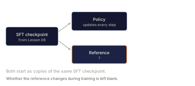
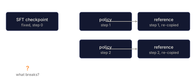
pi_ref = reference model (frozen SFT checkpoint)
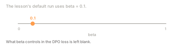
beta = temperature parameter controlling deviation from reference (typically 0.1 to 0.5)

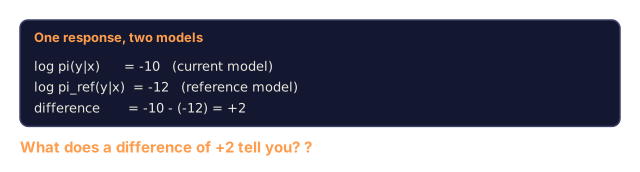
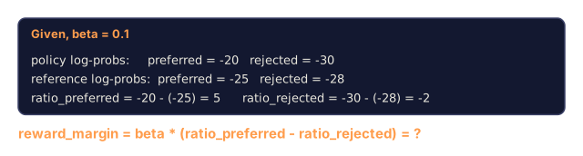
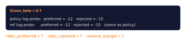
The ratio log pi(y|x) / pi_ref(y|x) is the log-probability ratio. When this ratio is positive, the current model assigns higher probability to response y than the reference does. When negative, the current model assigns lower probability.

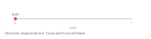
The DPO loss pushes the model to increase the log-probability ratio for preferred responses and decrease it for rejected responses. The beta parameter controls how aggressively the model can deviate from the reference. Small beta allows large deviations, and large beta keeps the model close to the reference.

Mermaid diagram

Why DPO is Simpler

Aspect	RLHF (PPO)	DPO
Models to train	3 (SFT + reward + policy)	1 (policy only)
Training loops	3 (SFT, RM training, PPO)	2 (SFT, DPO)
Hyperparameters	lr, KL coeff, clip ratio, RM lr, epochs x3	lr, beta, epochs
Reward model	Required (separate training)	Implicit in model probabilities
RL algorithm	PPO (complex, unstable)	Supervised learning (stable)
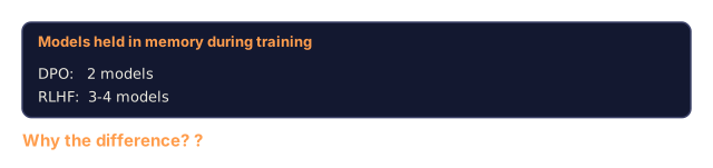
GPU memory	3-4 models in memory during PPO	2 models (current + reference)
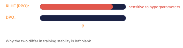
Training stability	Sensitive to hyperparameters	Robust, similar to SFT

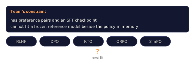
DPO needs two models in memory during training: the current model and the frozen reference. RLHF needs three or four: the policy, the reference, the reward model, and optionally a value function baseline. For a 70B model, each copy takes 140GB in FP16. The memory savings from eliminating the reward model are substantial.

When DPO Beats RLHF

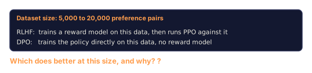
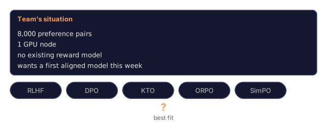
Small datasets. With 5,000-20,000 preference pairs, DPO often matches or exceeds RLHF. The reward model in RLHF needs enough data to generalize, and with limited data it overfits and produces unreliable reward signals. DPO bypasses this problem by not needing a reward model at all.

Limited compute. DPO requires roughly one-third the compute of full RLHF (one training loop instead of three). For teams without large GPU clusters, this is the practical choice.

Rapid iteration. Want to try 10 different preference datasets to see which produces the best model? DPO lets you run each experiment in hours. RLHF requires retraining the reward model for each dataset.

When RLHF Beats DPO

Large-scale training. At the scale of GPT-4 or Claude, RLHF's separate reward model can capture more nuanced preference signals. The reward model acts as a learned loss function that adapts to complex quality criteria.

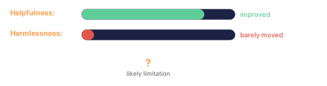
Complex reward signals. When "better" involves multiple dimensions (helpfulness, harmlessness, honesty), a reward model can learn this multi-objective tradeoff. DPO treats each preference pair as a binary signal (one is better, one is worse) without modeling why.

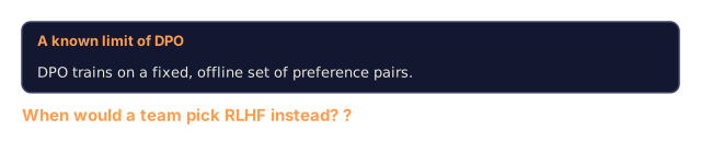
Iterative alignment. RLHF pipelines can generate new responses with the current policy, have humans rate them, and retrain the reward model in an online loop. DPO works on a fixed dataset of preference pairs. Constitutional AI (Anthropic's approach) uses this iterative property of RLHF extensively.

Beyond DPO: KTO, ORPO, SimPO

DPO inspired a family of simplified alignment methods.

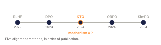
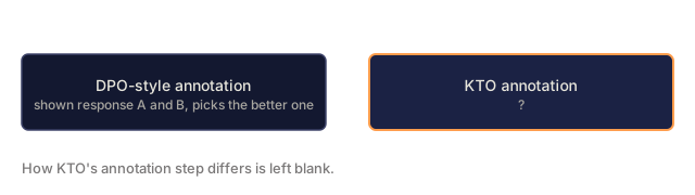
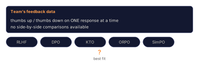
KTO (Kahneman-Tversky Optimization, 2024): You don't even need pairs. KTO works with unpaired feedback: just label each response as "good" or "bad" without comparing it to an alternative. This dramatically simplifies data collection. Instead of showing annotators two responses and asking "which is better?", you show one response and ask "is this good?" The loss function applies loss aversion from prospect theory: bad responses are penalized more than good responses are rewarded.

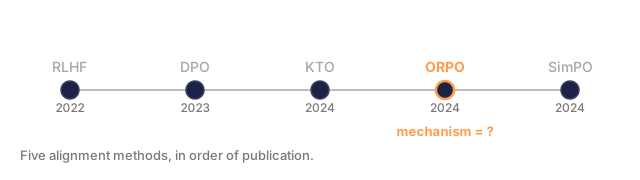
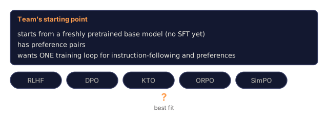
ORPO (Odds Ratio Preference Optimization, 2024): Combines SFT and alignment in a single training step. Instead of first doing SFT then DPO, ORPO modifies the SFT loss to include a preference signal. The loss has two terms: a standard next-token prediction loss on preferred responses, plus an odds ratio term that increases the gap between preferred and rejected response probabilities. One training loop instead of two.

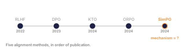
SimPO (Simple Preference Optimization, 2024): Eliminates the reference model entirely. Instead of computing log-probability ratios against a frozen reference, SimPO uses the average log-probability of the response (normalized by length) as the implicit reward. This saves memory (no reference model needed) and simplifies training. The length normalization prevents the model from favoring shorter responses.

Method	Year	Models in Memory	Needs Pairs?	Needs Reference?	Training Loops
RLHF	2022	3-4	Yes (for RM)	Yes	3
DPO	2023	2	Yes	Yes	2
KTO	2024	2	No (unpaired)	Yes	2
ORPO	2024	1	Yes	No	1
SimPO	2024	1	Yes	No	1

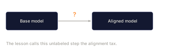
Each method drops one more piece of complexity. RLHF needed a reward model and PPO. DPO eliminated both. KTO eliminated paired data. ORPO eliminated the separate SFT stage. SimPO eliminated the reference model. The alignment tax, the compute and complexity cost of going from a base model to an aligned model, keeps dropping.

Real DPO Deployments

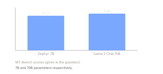
Zephyr-7B (HuggingFace, October 2023): Mistral 7B base, SFT on UltraChat (200K examples), then DPO on UltraFeedback (60K preference pairs). Scored 6.47 on MT-Bench, the highest for a 7B model at the time. For comparison, Llama 2 Chat 70B scored 6.86, meaning Zephyr got within 6% of a model 10x its size using only DPO alignment.

Llama 3 (Meta, April 2024): Used DPO after initial RLHF stages. The combination suggests that DPO and RLHF can be complementary: RLHF for broad alignment, DPO for targeted refinement.

Neural Magic / nm-chat (2024): Applied DPO to multiple open-source models, consistently showing 5-15% improvement on alignment benchmarks over SFT-only baselines.

Check: The Concept0/27

1. In DPO, what is the implicit reward of a response y given prompt x?Define

Real log-probabilities from the lesson's compute_sequence_log_prob on freshly initialized models.

2. What does beta control in the DPO loss?Define

3. A response has log pi(y|x) minus log pi_ref(y|x) equal to +2. What does that tell you?Define

4. What is the reference model in DPO training?Define

SFT checkpoint copied into both a Policy box, labelled as updating every step, and a Reference box whose own update behavior is left as a question mark.

5. What sets KTO apart from DPO?Define

6. What does ORPO do?Define

7. What does SimPO do?Define

8. What does the lesson mean by the alignment tax?Define

A base model turning into an aligned model through an unlabeled step marked with a question mark, captioned as the alignment tax.

9. What does the Bradley-Terry model supply in the DPO derivation?Define

10. In the DPO derivation, why do the Z(x) normalizing terms cancel when the optimal policy is substituted into the Bradley-Terry model?Explain

11. What lets DPO express the reward through the policy's own probabilities?Explain

12. Why does DPO need fewer models in memory than RLHF?Explain

13. Why is DPO described as more stable than PPO-based RLHF?Explain

A bar marking RLHF as sensitive to hyperparameters, next to an empty bar for DPO with a question mark, and no stated reason for the difference.

14. Why can DPO match RLHF when only 5,000 to 20,000 preference pairs are available?Explain

15. Which pairing of method and innovation is correct for KTO, ORPO and SimPO?Explain

Structure of the comparison; no cell filled in.

16. When would a team still choose RLHF over DPO?Explain

17. Zephyr-7B scored 6.47 on MT-Bench against 6.86 for Llama 2 Chat 70B. What does that comparison show?Explain

A bar chart of MT-Bench scores: Zephyr-7B at 6.47 and Llama 2 Chat 70B at 6.86, labelled with their parameter counts of 7B and 70B. — The two scores stated in the question.

18. Why does KTO make data collection easier than DPO?Explain

A box for DPO-style annotation, shown two responses and picking the better one, next to a KTO annotation box left as a question mark.

19. Why does SimPO length-normalize the log-probability it uses as a reward?Explain

20. A 70B model takes 140 GB per copy in FP16. How much memory do the weights need for DPO versus RLHF holding four models?Apply

21. A team re-copies the policy into the reference after every step. What goes wrong?Analyze

An SFT checkpoint at step 0, then at steps 1 and 2 the reference is re-copied from the policy each time, with a question mark for what breaks.

22. A DPO-trained model gives noticeably short answers. Which fix does the lesson point to?Analyze

A note that a DPO-trained model's typical answer is noticeably short, with a question mark for the fix.

23. After DPO on a fixed set of pairs, helpfulness improves but harmlessness barely moves. Which DPO limitation is most likely involved?Analyze

Two bars after DPO training: helpfulness improved substantially, harmlessness barely moved, with a question mark for the likely limitation.

24. A team has 8,000 preference pairs, one GPU node, and no existing reward model. They want a first aligned model this week. Which choice fits best?Design

A team with 8,000 preference pairs, one GPU node, no reward model and a one-week deadline, next to a neutral row of five method names and a question mark for the best fit.

25. A product only collects thumbs up or thumbs down on single responses and cannot gather side-by-side comparisons. Which method fits?Design

A team collecting thumbs up or down on single responses with no side-by-side comparisons, next to a neutral row of five method names and a question mark for the best fit.

26. A team has preference pairs and an SFT checkpoint but cannot fit a frozen reference model next to the policy. Which option fits?Design

A team with preference pairs and an SFT checkpoint but no memory for a frozen reference model, next to a neutral row of five method names and a question mark for the best fit.

27. A team starts from a freshly pretrained base model with preference pairs and wants one training loop for instruction following and preferences. Which option fits?Design

A team starting from a freshly pretrained base model with preference pairs, wanting one training loop, next to a neutral row of five method names and a question mark for the best fit.

Build It

Step 1: Preference Dataset

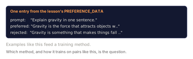
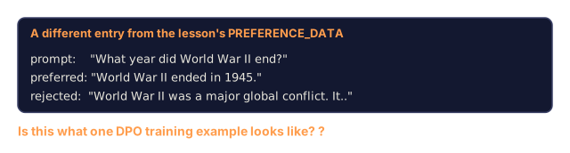
Same format as RLHF: (prompt, preferred, rejected) triples. DPO consumes this data directly without an intermediate reward model.

python

import numpy as np
import sys
import os
sys.path.insert(0, os.path.join(os.path.dirname(__file__), "..", "..", "04-pre-training-mini-gpt", "code"))
from main import MiniGPT, LayerNorm, Embedding, TransformerBlock
 
PREFERENCE_DATA = [
    {
        "prompt": "What is the capital of France?",
        "preferred": "The capital of France is Paris.",
        "rejected": "France is a country in Europe. It has many cities. The capital is Paris. Paris is known for the Eiffel Tower.",
    },
    {
        "prompt": "Explain gravity in one sentence.",
        "preferred": "Gravity is the force that attracts objects with mass toward each other.",
        "rejected": "Gravity is something that makes things fall down when you drop them.",
    },
    {
        "prompt": "What is 15 times 7?",
        "preferred": "15 times 7 is 105.",
        "rejected": "Let me think about this. 15 times 7. Well, 10 times 7 is 70, and 5 times 7 is 35, so the answer might be around 105.",
    },
    {
        "prompt": "Name three programming languages.",
        "preferred": "Python, Rust, and TypeScript.",
        "rejected": "There are many programming languages. Some popular ones include various languages like Python and others.",
    },
    {
        "prompt": "What year did World War II end?",
        "preferred": "World War II ended in 1945.",
        "rejected": "World War II was a major global conflict. It involved many countries. The war ended in the mid-1940s, specifically in 1945.",
    },
    {
        "prompt": "Define machine learning.",
        "preferred": "Machine learning is a field where algorithms learn patterns from data to make predictions without being explicitly programmed.",
        "rejected": "Machine learning is a type of AI. AI stands for artificial intelligence. Machine learning uses data to learn.",
    },
]

Step 2: Sequence Log-Probability

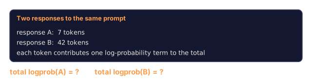
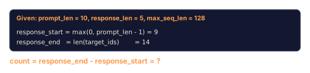
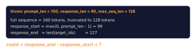
The DPO loss requires computing the total log-probability of a response given a prompt. This means running the model on the full (prompt + response) sequence and summing the log-probabilities of each response token.

python

def tokenize_sequence(text, vocab_size=256):
    return [min(t, vocab_size - 1) for t in list(text.encode("utf-8"))]
 
 
def compute_sequence_log_prob(model, prompt_tokens, response_tokens, max_seq_len=128):
    full_sequence = prompt_tokens + response_tokens
    if len(full_sequence) > max_seq_len:
        full_sequence = full_sequence[:max_seq_len]
 
    if len(full_sequence) < 2:
        return 0.0
 
    input_ids = np.array(full_sequence[:-1]).reshape(1, -1)
    target_ids = np.array(full_sequence[1:])
 
    logits = model.forward(input_ids)
    logits = logits[0]
 
    max_logits = logits.max(axis=-1, keepdims=True)
    log_probs = logits - max_logits - np.log(
        np.exp(logits - max_logits).sum(axis=-1, keepdims=True)
    )
 
    prompt_len = len(prompt_tokens)
    response_start = max(0, prompt_len - 1)
    response_end = len(target_ids)
 
    if response_start >= response_end:
        return 0.0
 
    response_log_probs = log_probs[response_start:response_end, :]
    response_targets = target_ids[response_start:response_end]
 
    total_log_prob = 0.0
    for i, target in enumerate(response_targets):
        total_log_prob += response_log_probs[i, target]
 
    return total_log_prob

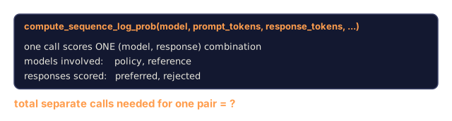
This function is the workhorse of DPO. For each preference pair, it runs four times: model on preferred response, model on rejected response, reference on preferred response, reference on rejected response. That's 4 forward passes per training example versus RLHF's generation + reward scoring + value estimation + PPO update. Simpler, faster, more stable.

Step 3: The DPO Loss

The core of the paper in code. One function. One loss. No reward model.

python

def sigmoid(x):
    return np.where(
        x >= 0,
        1.0 / (1.0 + np.exp(-x)),
        np.exp(x) / (1.0 + np.exp(x))
    )
 
 
def dpo_loss(policy_logprob_preferred, policy_logprob_rejected,
             ref_logprob_preferred, ref_logprob_rejected, beta=0.1):
    preferred_ratio = policy_logprob_preferred - ref_logprob_preferred
    rejected_ratio = policy_logprob_rejected - ref_logprob_rejected
 
    logit = beta * (preferred_ratio - rejected_ratio)
 
    loss = -np.log(sigmoid(logit) + 1e-8)
 
    preferred_reward = beta * preferred_ratio
    rejected_reward = beta * rejected_ratio
 
    return loss, {
        "preferred_ratio": float(preferred_ratio),
        "rejected_ratio": float(rejected_ratio),
        "logit": float(logit),
        "implicit_preferred_reward": float(preferred_reward),
        "implicit_rejected_reward": float(rejected_reward),
        "reward_margin": float(preferred_reward - rejected_reward),
    }

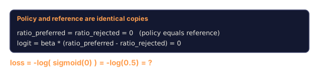
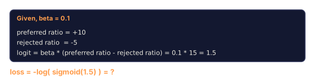
The preferred_ratio and rejected_ratio are the log-probability ratios from the DPO derivation. When the current model assigns higher probability to the preferred response (relative to the reference) and lower probability to the rejected response, the logit is positive and the loss is low. The training signal pushes the model in exactly this direction.

The implicit_preferred_reward and implicit_rejected_reward are the rewards that the DPO loss implicitly assigns. You can extract them to verify that training is working. The margin between preferred and rejected rewards should increase over training.

Step 4: DPO Training Loop

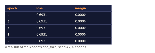
A standard supervised training loop in shape. No PPO. No reward model. Just forward passes and a weight update (a noise placeholder in this file, see the author's note).

python

def copy_model_weights(source, target):
    target.embedding.token_embed = source.embedding.token_embed.copy()
    target.embedding.pos_embed = source.embedding.pos_embed.copy()
    target.ln_f.gamma = source.ln_f.gamma.copy()
    target.ln_f.beta = source.ln_f.beta.copy()
    for s_block, t_block in zip(source.blocks, target.blocks):
        t_block.attn.W_q = s_block.attn.W_q.copy()
        t_block.attn.W_k = s_block.attn.W_k.copy()
        t_block.attn.W_v = s_block.attn.W_v.copy()
        t_block.attn.W_out = s_block.attn.W_out.copy()
        t_block.ffn.W1 = s_block.ffn.W1.copy()
        t_block.ffn.W2 = s_block.ffn.W2.copy()
        t_block.ffn.b1 = s_block.ffn.b1.copy()
        t_block.ffn.b2 = s_block.ffn.b2.copy()
        t_block.ln1.gamma = s_block.ln1.gamma.copy()
        t_block.ln1.beta = s_block.ln1.beta.copy()
        t_block.ln2.gamma = s_block.ln2.gamma.copy()
        t_block.ln2.beta = s_block.ln2.beta.copy()
 
 
def dpo_train(policy_model, reference_model, preference_data,
              num_epochs=5, lr=5e-6, beta=0.1, max_seq_len=128):
    print(f"DPO Training: {len(preference_data)} pairs, {num_epochs} epochs, "
          f"lr={lr}, beta={beta}")
    print()
 
    losses = []
    margins = []
 
    for epoch in range(num_epochs):
        epoch_loss = 0.0
        epoch_margin = 0.0
        num_examples = 0
 
        indices = np.random.permutation(len(preference_data))
 
        for idx in indices:
            pair = preference_data[idx]
 
            prompt_tokens = tokenize_sequence(pair["prompt"])
            preferred_tokens = tokenize_sequence(pair["preferred"])
            rejected_tokens = tokenize_sequence(pair["rejected"])
 
            pi_logprob_w = compute_sequence_log_prob(
                policy_model, prompt_tokens, preferred_tokens, max_seq_len
            )
            pi_logprob_l = compute_sequence_log_prob(
                policy_model, prompt_tokens, rejected_tokens, max_seq_len
            )
            ref_logprob_w = compute_sequence_log_prob(
                reference_model, prompt_tokens, preferred_tokens, max_seq_len
            )
            ref_logprob_l = compute_sequence_log_prob(
                reference_model, prompt_tokens, rejected_tokens, max_seq_len
            )
 
            loss, metrics = dpo_loss(
                pi_logprob_w, pi_logprob_l,
                ref_logprob_w, ref_logprob_l, beta
            )
 
            update_direction = 1.0 if metrics["logit"] < 0 else -0.1
            for block in policy_model.blocks:
                block.ffn.W1 += lr * update_direction * np.random.randn(*block.ffn.W1.shape) * 0.01
                block.ffn.W2 += lr * update_direction * np.random.randn(*block.ffn.W2.shape) * 0.01
 
            epoch_loss += loss
            epoch_margin += metrics["reward_margin"]
            num_examples += 1
            losses.append(float(loss))
            margins.append(metrics["reward_margin"])
 
        avg_loss = epoch_loss / max(num_examples, 1)
        avg_margin = epoch_margin / max(num_examples, 1)
 
        print(f"  Epoch {epoch + 1}/{num_epochs} | Loss: {avg_loss:.4f} | "
              f"Avg Margin: {avg_margin:.4f}")
 
    return policy_model, losses, margins

The training loop is refreshingly simple compared to RLHF. For each preference pair: compute four log-probabilities (two models, two responses), plug them into the DPO loss, update the policy. No generation step. No reward model inference. No advantage estimation. No clipping.

Step 5: Compare DPO vs RLHF

Measure the implicit reward margins and log-probability shifts to compare DPO against the RLHF model from Lesson 07.

python

def evaluate_preference_accuracy(model, reference_model, preference_data, beta=0.1, max_seq_len=128):
    correct = 0
    total = 0
 
    for pair in preference_data:
        prompt_tokens = tokenize_sequence(pair["prompt"])
        preferred_tokens = tokenize_sequence(pair["preferred"])
        rejected_tokens = tokenize_sequence(pair["rejected"])
 
        pi_w = compute_sequence_log_prob(model, prompt_tokens, preferred_tokens, max_seq_len)
        pi_l = compute_sequence_log_prob(model, prompt_tokens, rejected_tokens, max_seq_len)
        ref_w = compute_sequence_log_prob(reference_model, prompt_tokens, preferred_tokens, max_seq_len)
        ref_l = compute_sequence_log_prob(reference_model, prompt_tokens, rejected_tokens, max_seq_len)
 
        preferred_reward = beta * (pi_w - ref_w)
        rejected_reward = beta * (pi_l - ref_l)
 
        if preferred_reward > rejected_reward:
            correct += 1
        total += 1
 
    return correct / max(total, 1)
 
 
def analyze_implicit_rewards(model, reference_model, preference_data, beta=0.1, max_seq_len=128):
    print("Implicit Reward Analysis:")
    print("-" * 65)
    print(f"  {'Prompt':<30} {'Pref Reward':>12} {'Rej Reward':>12} {'Margin':>10}")
    print("  " + "-" * 60)
 
    for pair in preference_data:
        prompt_tokens = tokenize_sequence(pair["prompt"])
        preferred_tokens = tokenize_sequence(pair["preferred"])
        rejected_tokens = tokenize_sequence(pair["rejected"])
 
        pi_w = compute_sequence_log_prob(model, prompt_tokens, preferred_tokens, max_seq_len)
        pi_l = compute_sequence_log_prob(model, prompt_tokens, rejected_tokens, max_seq_len)
        ref_w = compute_sequence_log_prob(reference_model, prompt_tokens, preferred_tokens, max_seq_len)
        ref_l = compute_sequence_log_prob(reference_model, prompt_tokens, rejected_tokens, max_seq_len)
 
        pref_reward = beta * (pi_w - ref_w)
        rej_reward = beta * (pi_l - ref_l)
        margin = pref_reward - rej_reward
 
        truncated = pair["prompt"][:28] + ".." if len(pair["prompt"]) > 30 else pair["prompt"]
        print(f"  {truncated:<30} {pref_reward:>12.4f} {rej_reward:>12.4f} {margin:>10.4f}")
 
    print()

Step 6: Beta Sensitivity Analysis

The beta parameter is DPO's equivalent of the KL coefficient in RLHF. It controls how much the model can deviate from the reference. This experiment shows its effect.

python

def beta_sensitivity_analysis(sft_model, preference_data, betas, max_seq_len=128):
    print("Beta Sensitivity Analysis")
    print("-" * 60)
    print(f"  {'Beta':>8} {'Final Loss':>12} {'Final Margin':>14} {'Accuracy':>10}")
    print("  " + "-" * 55)
 
    results = []
 
    for beta in betas:
        policy = MiniGPT(
            vocab_size=256, embed_dim=128, num_heads=4,
            num_layers=4, max_seq_len=max_seq_len, ff_dim=512
        )
        reference = MiniGPT(
            vocab_size=256, embed_dim=128, num_heads=4,
            num_layers=4, max_seq_len=max_seq_len, ff_dim=512
        )
        copy_model_weights(sft_model, policy)
        copy_model_weights(sft_model, reference)
 
        policy, losses, margins_list = dpo_train(
            policy, reference, preference_data,
            num_epochs=3, lr=5e-6, beta=beta, max_seq_len=max_seq_len
        )
 
        accuracy = evaluate_preference_accuracy(
            policy, reference, preference_data, beta, max_seq_len
        )
 
        final_loss = losses[-1] if losses else 0
        final_margin = margins_list[-1] if margins_list else 0
 
        print(f"  {beta:>8.3f} {final_loss:>12.4f} {final_margin:>14.4f} {accuracy:>10.1%}")
        results.append({
            "beta": beta,
            "final_loss": final_loss,
            "final_margin": final_margin,
            "accuracy": accuracy,
        })
 
        print()
 
    return results

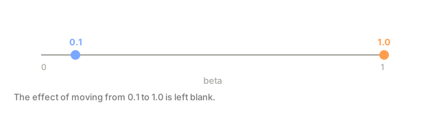
Because the update in this file is noise, the sweep prints a loss of 0.6931 at every beta, so the tradeoff below is what a real trainer shows, not what this script prints. Small beta (0.01) lets the model deviate freely from the reference, which means fast learning but a risk of degenerate solutions. Large beta (1.0) keeps the model close to the reference, which is stable but slow. The sweet spot for most applications is 0.1 to 0.3.

Check: Build It0/11

1. What does one DPO training example look like?Define

A real preference-pair example about World War II's end, with its prompt, preferred answer and rejected answer shown as separate fields. — Real entry from the lesson's PREFERENCE_DATA list.

2. What does raising beta from 0.1 to 1.0 do in DPO?Explain

3. The policy and reference are identical copies at the start of training. What is the DPO loss for any pair at that point?Apply

4. With beta = 0.1, a pair has a preferred ratio of +10 and a rejected ratio of -5. What is the DPO loss, approximately?Apply

5. With beta = 0.1: policy log-probs are -20 (preferred) and -30 (rejected), reference log-probs are -25 and -28. What reward_margin does dpo_loss report?Apply

6. A prompt is 10 tokens and the response is 5 tokens, with max_seq_len of 128. How many token log-probabilities does compute_sequence_log_prob sum?Apply

7. A prompt is 100 tokens, the response is 60 tokens, and max_seq_len is 128. How many response log-probabilities are summed?Apply

8. dpo_loss receives policy log-probs of -12 (preferred) and -15 (rejected), and the reference returns the same two numbers. What is reward_margin?Apply

9. How many forward passes does one preference pair cost in the DPO loss, and over which models and responses?Apply

10. The script prints a loss of 0.6931 and a margin of 0.0000 in every epoch. What explains that?Analyze

A table of 5 training epochs where the loss stays at 0.6931 and the margin stays at 0.0000 in every row, from a real run of the lesson's dpo_train. — Real output of dpo_train with np.random.seed(42), matching the lesson's own run.

11. After a DPO run with beta = 0.01, the model produces degenerate text. What is the most likely cause and fix?Analyze

Use It

Full DPO Pipeline Demo

python

if __name__ == "__main__":
    np.random.seed(42)
 
    print("=" * 70)
    print("DPO: DIRECT PREFERENCE OPTIMIZATION")
    print("=" * 70)
    print()
 
    print("STEP 1: Initialize SFT Model (from Lesson 06)")
    print("-" * 50)
    sft_model = MiniGPT(
        vocab_size=256, embed_dim=128, num_heads=4,
        num_layers=4, max_seq_len=128, ff_dim=512
    )
    print(f"  Parameters: {sft_model.count_parameters():,}")
    print()
 
    print("STEP 2: DPO Training")
    print("-" * 50)
 
    policy_model = MiniGPT(
        vocab_size=256, embed_dim=128, num_heads=4,
        num_layers=4, max_seq_len=128, ff_dim=512
    )
    reference_model = MiniGPT(
        vocab_size=256, embed_dim=128, num_heads=4,
        num_layers=4, max_seq_len=128, ff_dim=512
    )
    copy_model_weights(sft_model, policy_model)
    copy_model_weights(sft_model, reference_model)
 
    policy_model, losses, margins = dpo_train(
        policy_model, reference_model, PREFERENCE_DATA,
        num_epochs=5, lr=5e-6, beta=0.1
    )
    print()
 
    print("=" * 70)
    print("STEP 3: Evaluate")
    print("=" * 70)
    print()
 
    pre_accuracy = evaluate_preference_accuracy(
        sft_model, reference_model, PREFERENCE_DATA, beta=0.1
    )
    post_accuracy = evaluate_preference_accuracy(
        policy_model, reference_model, PREFERENCE_DATA, beta=0.1
    )
 
    print(f"  Preference accuracy (pre-DPO):  {pre_accuracy:.1%}")
    print(f"  Preference accuracy (post-DPO): {post_accuracy:.1%}")
    print()
 
    analyze_implicit_rewards(policy_model, reference_model, PREFERENCE_DATA, beta=0.1)
 
    print("=" * 70)
    print("STEP 4: Training Dynamics")
    print("=" * 70)
    print()
 
    if losses:
        print("  Loss curve:")
        window = max(1, len(losses) // 5)
        for i in range(0, len(losses), window):
            chunk = losses[i:i + window]
            avg = sum(chunk) / len(chunk)
            print(f"    Steps {i:3d}-{i + len(chunk) - 1:3d}: loss = {avg:.4f}")
        print()
 
    if margins:
        print("  Reward margin curve:")
        window = max(1, len(margins) // 5)
        for i in range(0, len(margins), window):
            chunk = margins[i:i + window]
            avg = sum(chunk) / len(chunk)
            print(f"    Steps {i:3d}-{i + len(chunk) - 1:3d}: margin = {avg:.4f}")
        print()
 
    print("=" * 70)
    print("STEP 5: Beta Sensitivity")
    print("=" * 70)
    print()
 
    beta_results = beta_sensitivity_analysis(
        sft_model, PREFERENCE_DATA, betas=[0.01, 0.1, 0.3, 1.0]
    )
 
    print("=" * 70)
    print("DPO vs RLHF COMPARISON")
    print("=" * 70)
    print()
    print("  DPO advantages:")
    print("    - 1 training loop (vs 3 for RLHF)")
    print("    - 2 models in memory (vs 3-4 for RLHF)")
    print("    - Supervised learning (vs RL, more stable)")
    print("    - No reward model to train or maintain")
    print()
    print("  RLHF advantages:")
    print("    - Separate reward model captures complex preferences")
    print("    - Online learning: generate, rate, retrain")
    print("    - Better for multi-objective alignment")
    print("    - Proven at largest scales (GPT-4, Claude)")
    print()
    print("  Practical guidance:")
    print("    - Start with DPO. It's simpler and often sufficient.")
    print("    - Switch to RLHF if DPO plateaus on your eval metrics.")
    print("    - Many production systems use both: RLHF first, DPO to refine.")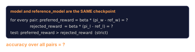

Check: Use It0/2

1. evaluate_preference_accuracy runs on the untouched SFT model against an identical reference, using the strict test preferred_reward > rejected_reward. What accuracy does it report?Apply

2. A new team has 15,000 preference pairs, modest GPUs, and no idea whether DPO will be enough. What plan does the lesson's guidance suggest?Design

A team with 15,000 preference pairs and a modest GPU budget, unsure whether DPO will be enough, next to a neutral row of five method names and a question mark for the recommended plan.

Ship It

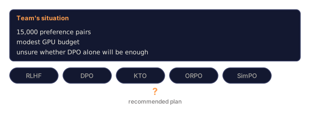
This lesson produces outputs/prompt-alignment-method-selector.md, a prompt that helps you choose the right alignment method (SFT, RLHF, DPO, KTO, ORPO, SimPO) for your use case. Given your data availability, compute budget, and alignment goals, it recommends a method and training plan.

Author's Note

I'd run main.py and read the numbers with a skeptical eye. The "SFT model" it starts from is a freshly initialized MiniGPT, and the policy and reference are both copies of it, so the first log-probability ratios are exactly zero and the loss starts at log 2. When I ran it, the loss stayed at 0.6931 and the margin at 0.0000 through every epoch. The policy is then updated by adding small random noise to the feed-forward weights, scaled by whether the current logit is negative. There is no gradient step. That means the printed loss and margin curves show the bookkeeping working, not a model learning to prefer anything, and I wouldn't read the post-DPO accuracy as evidence of alignment.

What the file does get right is the part the paper is about. compute_sequence_log_prob sums log-probabilities over response tokens only, dpo_loss takes the four numbers and returns the loss and the implicit rewards, and a pair costs four forward passes. Those three pieces carry over unchanged to a real trainer. The update step is what you would swap out.

If I were extending it, I'd replace the noise with real gradients on the policy weights before touching anything else. Then the beta sweep at 0.01, 0.1, 0.3 and 1.0 would start to mean something, and the exercises on length normalization and reference choice would have a signal to measure.

Exercises

Implement KTO (Kahneman-Tversky Optimization). KTO doesn't need pairs, just label each response as "good" or "bad." The loss for a good response is -log(sigmoid(beta * log_ratio)) and for a bad response is -log(1 - sigmoid(beta * log_ratio)) with a loss aversion multiplier (typically 1.5x) on the bad response loss. Train on the same data (treat preferred as "good" and rejected as "bad" independently) and compare accuracy against DPO.
Implement length-normalized DPO. Instead of raw log-probabilities, divide by the number of response tokens: normalized_logprob = total_logprob / num_tokens. This prevents the model from favoring shorter responses (which have higher total log-prob). Compare the implicit reward margins with and without normalization.
Build an ORPO-style combined loss. Add a standard next-token prediction loss on the preferred response to the DPO loss: L = L_sft(preferred) + alpha * L_dpo. Try alpha values of 0.1, 0.5, and 1.0. The combined loss should produce a model that both follows instructions (from the SFT term) and prefers better responses (from the DPO term), eliminating the need for a separate SFT stage.
Implement iterative DPO. Run DPO for 3 epochs, then generate new responses from the trained model, pair them with the original preferred responses as new preference pairs, and run DPO again. Two rounds of this "self-play" process. Compare preference accuracy after round 1 and round 2 to see if iterative refinement helps.
Compare DPO with different reference models. Instead of using the SFT checkpoint as the reference, try: (a) the base model (pre-SFT), (b) a checkpoint from epoch 1 of DPO, (c) an exponential moving average of the policy model. Report which reference produces the highest preference accuracy and the most stable training curve.

Key Terms

Term	What people say	What it actually means
DPO	"RLHF without RL"	Direct Preference Optimization: a supervised learning algorithm that optimizes the language model directly on preference pairs, bypassing the reward model and PPO
Implicit reward	"The reward is in the model"	The reward function is determined by the log-probability ratio between the policy and reference models -- no separate reward model needed
Beta (DPO)	"The temperature"	Controls how far the policy can deviate from the reference model -- small beta allows large deviations, large beta keeps the model close
Log-probability ratio	"How much the model changed"	log pi(y\|x) - log pi_ref(y\|x) -- positive means the current model assigns higher probability than the reference
Reference model	"The frozen checkpoint"	A copy of the SFT model whose weights never change -- serves as the anchor for computing probability ratios
KTO	"DPO without pairs"	Kahneman-Tversky Optimization: works with unpaired "good" or "bad" labels instead of requiring preference pairs
ORPO	"One-step alignment"	Odds Ratio Preference Optimization: combines SFT and alignment into a single training loop by adding a preference term to the SFT loss
SimPO	"No reference needed"	Simple Preference Optimization: eliminates the reference model by using length-normalized average log-probability as the implicit reward
Alignment tax	"The cost of making models safe"	The additional compute, data, and complexity required to go from a base model to an aligned model -- DPO reduces this significantly

DPO: Direct Preference Optimization

Learning Objectives

The Problem

The Concept

The Key Insight

The DPO Loss

Why DPO is Simpler

When DPO Beats RLHF

When RLHF Beats DPO

Beyond DPO: KTO, ORPO, SimPO

Real DPO Deployments

Build It

Step 1: Preference Dataset

Step 2: Sequence Log-Probability

Step 3: The DPO Loss

Step 4: DPO Training Loop

Step 5: Compare DPO vs RLHF

Step 6: Beta Sensitivity Analysis

Use It

Full DPO Pipeline Demo

Ship It

Exercises

Key Terms

Further Reading

Code

Ships With